Analysis Guide Part IV
Subsetting and subclustering with SpatialMap
AnalysisGuide4_Subsetting_and_subclustering.RmdNavigate vignettes
Introduction
In the first round of unsupervised clustering and cell phenotyping, we were able to identify several phenotypes of interest. We focused on a subset of the biomarker panel in the first round, in order to assign broader cell phenotypes with high confidence and minimal interference from biomarkers that are expressed across multiple clusters. However, since we focused on a subset of biomarkers in the first round of clustering, we weren’t able to dissect some cell types in the full depth possible with the panel.
In this vignette, the we will walk through subsetting the SpatialMap object, subclustering to identify more detailed phenotypes, and assigning these subcluster labels back to the parent object. We will focus on deeper phenotyping of the macrophage cluster.
For a detailed tutorial on subset and slice operations in SpatialMap and Region objects, please see the tutorial vignette on manipulating SpatialMap objects.
To start, let’s read the data from the previous vignettes.
data_file <- "sm_post_clustering.RDS"

data_dir <- "."
# facil::check_dir is useful if you're running this yourself on code ocean
rw_paths <- facil::check_dir(data_dir)

sm <- readRDS(file.path(rw_paths$read_dir, data_file))
You can recreate this analysis yourself on Code Ocean by attaching the “SpatialMap vignettes” data asset to your capsule and changing
data_dirto/data/spatialmap_vignettes/spatialmap_analysis_guides/
Subsetting cells
You can easily subset SpatialMap objects by regions, cell IDs, or clusters of cells defined in the cell metadata, using the function .smsubset.
First, you can check the options by looking at the cellMetadata slot for sm.
cellMetadata(sm)$first_round_clustering %>% unique() %>% sort()
#>  [1] "B cells"                    "CD4+ T cells"
#>  [3] "CD8+ T cells"               "Dendritic cells"
#>  [5] "Epithelium"                 "Langerhans cells"
#>  [7] "Macrophages"                "Mast cells"
#>  [9] "Other"                      "T regs"
#> [11] "Vascular endothelial cells" "Vimentin+ Stroma"
Next, select which clusters you’d like to perform sub-phenotyping on and subset the sm object using smSubset
sm_macs <- smSubset(sm, on = "first_round_clustering", keep = "Macrophages")To check whether subsetting was successful, you can check the number of cells in the parent and subsetted object.
Subclustering
Now, we can subcluster, this time at a higher resolution, to try to make out subpopulations. As with the first round clustering, we can define biomarkers of interest for sub-phenotyping macrophages.
Similarly to when we clustered the full dataset, running UMAP may run more quickly if you run it in a session with more CPUs, which enables parallel processing. This is often less of a concern with subclustering, because the number of cells is much smaller
mac_clustering_features <- c(
"CD163", # Polarization
"CD68", # Canonical macrophage markers
"CD11c", # Separate out contaminating dendritic cells
"HLA-DR", # Activation
"PDL1" # Immunoregulatory state
)
set.seed(2142)
# Cluster on subset
sm_macs <- sm_macs %>%
runUMAP(data.slot = "ScaledData",
PCA = F, # Omitting PCA because there are only a few features already
features = mac_clustering_features) %>%
clusterCells(cluster.resolution = 0.5)
#> By analysis: 'combined'
#>
#> Computing UMAP
#>
#> 16:02:28 UMAP embedding parameters a = 0.9922 b = 1.112
#> 16:02:28 Read 2685 rows and found 5 numeric columns
#> 16:02:29 Building Annoy index with metric = cosine, n_trees = 50
#> 0% 10 20 30 40 50 60 70 80 90 100%
#> [----|----|----|----|----|----|----|----|----|----|
#> **************************************************|
#> 16:02:29 Writing NN index file to temp file /tmp/Rtmptnmd5W/filef8b117abfd5
#> 16:02:29 Searching Annoy index using 2 threads, search_k = 3000
#> 16:02:30 Annoy recall = 100%
#> 16:02:30 Commencing smooth kNN distance calibration using 2 threads with target n_neighbors = 30
#> 16:02:31 Initializing from normalized Laplacian + noise (using irlba)
#> 16:02:31 Commencing optimization for 500 epochs, with 100332 positive edges
#> 16:02:34 Optimization finished
#> By analysis: 'combined'
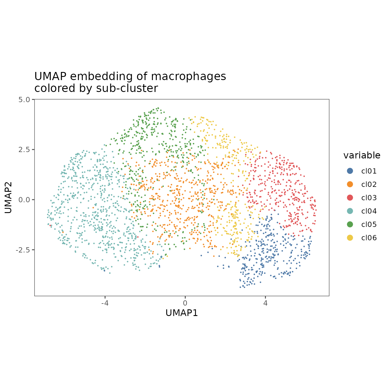
#> We can visualize the results in a similar way to what we did with the first round of clustering. We can start with a UMAP.
plotRepresentation(
  sm_macs,
  representation = "umap",
  what = ".clusters",
  plot.title = "UMAP embedding of macrophages\ncolored by sub-cluster"
)
#>   By analysis: 'combined'
#> 
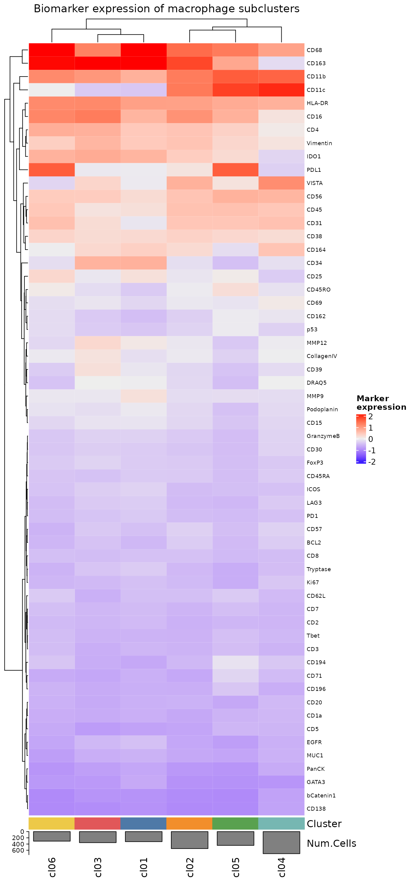
We can also make some heatmap visualizations, both with all biomarkers,
plotExpressionHeatmap(
  sm_macs,
  summary.fun = "median",
  summarize.across = ".clusters",
  # Plotting with the original scaled data shows biomarker expression
  # values relative to the whole dataset
  # rather than emphasizing differences between macrophage clusters.
  data.slot = "ScaledData",
  scaling = "none",
  column_title = "Biomarker expression of macrophage subclusters"
)
#> Plotting expression from slot 'ScaledData'.
#> Scaling = 'none'
#>   By analysis: 'combined'
#> 
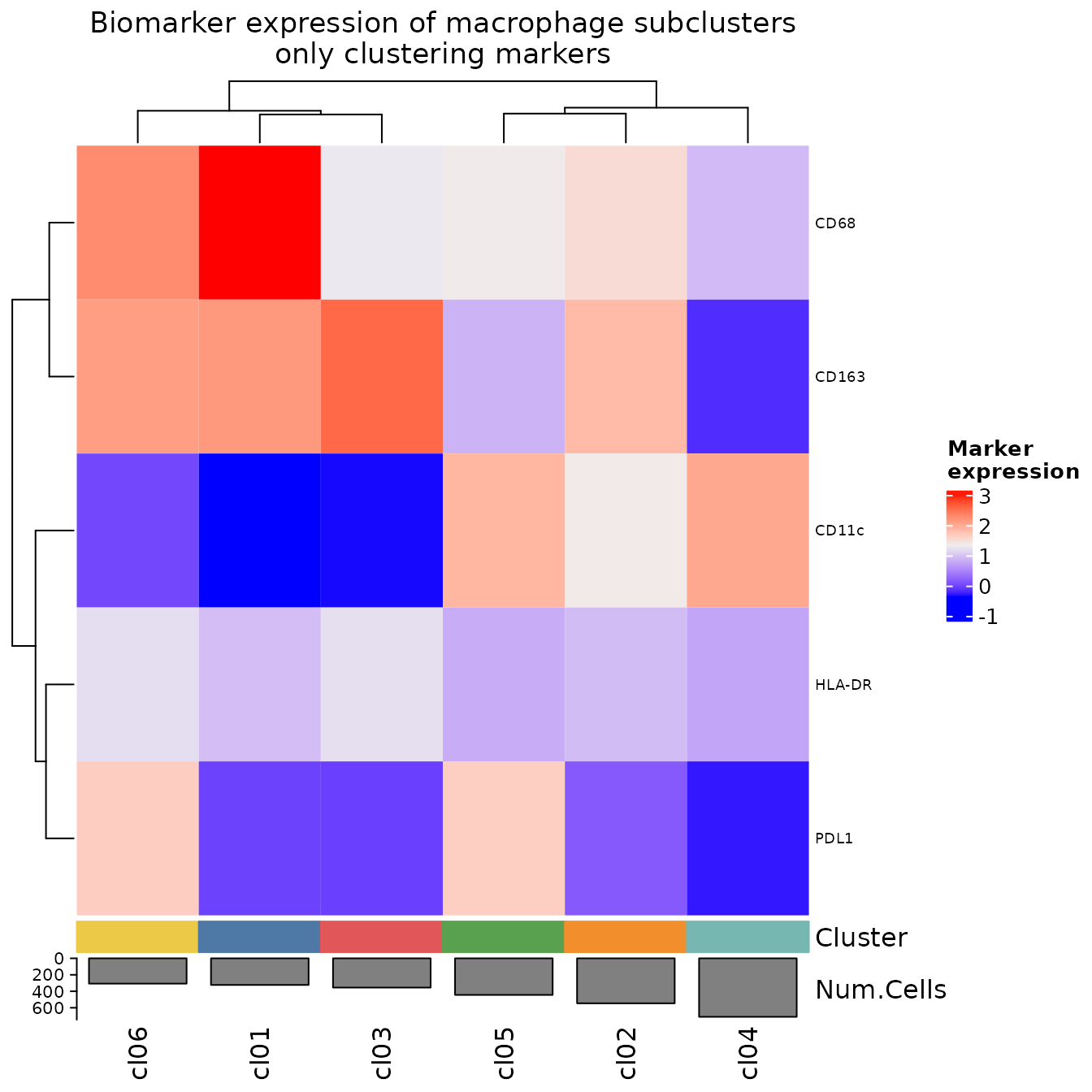
and with just the biomarkers used for sub-clustering.
all_markers <- features(sm_macs)

exclude_markers <- all_markers[!(all_markers %in% mac_clustering_features)]

plotExpressionHeatmap(
  sm_macs,
  summary.fun = "median",
  summarize.across = ".clusters",
  data.slot = "ScaledData",
  scaling = "none",
  column_title = "Biomarker expression of macrophage subclusters\nonly clustering markers",
  exclude.markers = exclude_markers
)
#> Plotting expression from slot 'ScaledData'.
#> Scaling = 'none'
#>   By analysis: 'combined'
#> 
We then annotate the clusters as before. Here, we’re following the example set in the paper that is the source of this dataset.
As with the first tier of clustering, it can often be helpful to push this annotation set to the Portal and generate a visualizer overlay. If your goal is to use this phenotyping for analysis on the portal, it makes sense to also associate it with the QC filter you generated in Analysis Guide 2. This process is described in the tutorial vignette Pushing annotations to the Portal. The Insights app may also be useful here, as it was with the first tier of clustering. More information on how to utilize the Insights app in conjunction with Workbench is in the tutorial vignette Pushing plots to the Portal.
phenotype_column_name <- "labeled_macrophage_subclusters"

# Assign your clusters to phenotypes here
# Clusters with the same name will be "merged"
cluster.labels <- c(
  cl01 = "M1 > M2",
  cl02 = "M1 > M2 CD11c+",
  cl03 = "M2 > M1",
  cl04 = "PDL1+",
  cl05 = "M2 > M1",
  cl06 = "APCs"
)

mapped.vals <- mapValues(as.character(cellMetadata(sm_macs)$.clusters), cluster.labels)
sm_macs <- sm_macs %>% addCellMetadata(mapped.vals, col.names = phenotype_column_name)
Mapping
After annotating the subclusters, we can also map these values back to the original object.
names(mapped.vals) <- cellMetadata(sm_macs)$cell.id

original_clusters <- cellMetadata(sm)$first_round_clustering
names(original_clusters) <- cellMetadata(sm)$cell.id

# Using cell.id as a key, we replace the annotation of cells that
# have been analyzed here with the more detailed subcluster labels
original_clusters[names(mapped.vals)] <- mapped.vals

sm <- addCellMetadata(sm, original_clusters, "clustering_with_macrophage_subtypes")
You can check that this augmentation was successful by inspecting the cellMetadata slot of the parent sm object.
cellMetadata(sm)$clustering_with_macrophage_subtypes %>% unique() %>% sort()
#>  [1] "APCs"                       "B cells"
#>  [3] "CD4+ T cells"               "CD8+ T cells"
#>  [5] "Dendritic cells"            "Epithelium"
#>  [7] "Langerhans cells"           "M1 > M2"
#>  [9] "M1 > M2 CD11c+"             "M2 > M1"
#> [11] "Mast cells"                 "Other"
#> [13] "PDL1+"                      "T regs"
#> [15] "Vascular endothelial cells" "Vimentin+ Stroma"
You can see that the “Macrophage” annotation is gone, and has been replaced with the various subclusters defined in this analysis.
Although we demonstrated subclustering only one of the parent clusters in this object, it may be useful to subcluster others as well. T-cells, for instance, are a cell type with a number of subpopulations that can be defined by biomarkers in our standard 51-plex panel.
We can now save our results and get to the really interesting part of the analysis guide: spatial analyses.