Tutorial: Manipulating SpatialMap Objects
Tutorial_Manipulating_SpatialMap_objects.Rmd
library(facil)
library(SpatialMap)
Basic operations
Subset, merge, and group
To get started quickly, let’s load a toy SpatialMap (sm_tonsil) object containing CODEX data.
sm_tonsil <- load_sm_data("tonsil")SpatialMap (SM) provides some simple functions to make it easier to cut your data or conduct grouped analyses.
Subset
Users may want to subset SM objects by removing regions from their analysis. They might also want to subset their object based on cells or cell metadata, e.g. if they want to pull out only one or more cell classes for further analysis. Both are easily accomplished with somewhat different syntaxes. By Regions:
## Keep only specific Regions.
## You can index Regions numerically or by name.
## This works just like base R.

sm2 <- sm_tonsil[2]
sm2
#> SpatialMap object
#> Active analysis:  regions
#> +  10,694 total cells
#> +  16 features
#> +  1 Regions:
#>   - TonsilB
sm2 <- sm_tonsil["TonsilA"]
sm2
#> SpatialMap object
#> Active analysis:  regions
#> +  5,810 total cells
#> +  16 features
#> +  1 Regions:
#>   - TonsilA
And by cell annotations: (note: for the purposes of this demo, I am saving subset outputs to a new SM object, but that isn’t strictly necessary.)
## First, let's make some toy annotations

toy <- sample(letters, size = length(cells(sm_tonsil)), replace = T)

sm_tonsil <- addCellMetadata(sm_tonsil, toy, col.names = "some_letters")

## Now subset by the cell annotations

sm2 <- smSubset(sm_tonsil, on = "some_letters", keep = letters[1:10])
head(cellMetadata(sm_tonsil)) ## Note we only see the first part of the alphabet in the metadata now
#>                cell_id        cell.id anno316_some_categories anno916_Leiden_v1
#> TonsilA.125182  125182 TonsilA.125182                     yay         Cluster 2
#> TonsilA.125238  125238 TonsilA.125238                     nay         Cluster 2
#> TonsilA.125254  125254 TonsilA.125254                     yay         Cluster 1
#> TonsilA.125325  125325 TonsilA.125325                     yay         Cluster 1
#> TonsilA.125326  125326 TonsilA.125326                     nay         Cluster 6
#> TonsilA.125608  125608 TonsilA.125608                     nay         Cluster 1
#>                anno248_test_subset_annotation_324
#> TonsilA.125182                                  p
#> TonsilA.125238                                  u
#> TonsilA.125254                                  t
#> TonsilA.125325                                  t
#> TonsilA.125326                                  b
#> TonsilA.125608                                  y
#>                anno1189_uqc_test10_letters_qc_assoc anno1149_uqc_test10_letters
#> TonsilA.125182                                    b                           b
#> TonsilA.125238                                    b                           b
#> TonsilA.125254                                    b                           b
#> TonsilA.125325                                    c                           c
#> TonsilA.125326                                    c                           c
#> TonsilA.125608                                    b                           b
#>                anno1133_uqc_test03_letters anno247_test_letters_324
#> TonsilA.125182                           l                        p
#> TonsilA.125238                           k                        u
#> TonsilA.125254                           z                        t
#> TonsilA.125325                           f                        t
#> TonsilA.125326                           f                        b
#> TonsilA.125608                           m                        y
#>                anno1190_uqc_test10_letters_qc_assoc_postfilt
#> TonsilA.125182                                          <NA>
#> TonsilA.125238                                          <NA>
#> TonsilA.125254                                             b
#> TonsilA.125325                                          <NA>
#> TonsilA.125326                                          <NA>
#> TonsilA.125608                                          <NA>
#>                anno253_Hierarchy.1 anno1797_uqc_test10_letters_221213
#> TonsilA.125182              not Th                                  c
#> TonsilA.125238              not Th                                  b
#> TonsilA.125254    Epithelial Cells                                  b
#> TonsilA.125325    Epithelial Cells                                  b
#> TonsilA.125326   Endothelial Cells                                  b
#> TonsilA.125608    Epithelial Cells                                  b
#>                anno254_Neighborhood.clustering.based.on.annotation.set.253
#> TonsilA.125182                                              neighborhood_2
#> TonsilA.125238                                              neighborhood_2
#> TonsilA.125254                                              neighborhood_0
#> TonsilA.125325                                              neighborhood_0
#> TonsilA.125326                                              neighborhood_2
#> TonsilA.125608                                              neighborhood_0
#>                anno1145_uqc_test08_letters anno1143_uqc_test08_letters  Region
#> TonsilA.125182                           l                           l TonsilA
#> TonsilA.125238                           k                           k TonsilA
#> TonsilA.125254                           z                           z TonsilA
#> TonsilA.125325                           f                           f TonsilA
#> TonsilA.125326                           f                           f TonsilA
#> TonsilA.125608                           m                           m TonsilA
#>                    color width n_channels height
#> TonsilA.125182 grayscale  9408          4   9072
#> TonsilA.125238 grayscale  9408          4   9072
#> TonsilA.125254 grayscale  9408          4   9072
#> TonsilA.125325 grayscale  9408          4   9072
#> TonsilA.125326 grayscale  9408          4   9072
#> TonsilA.125608 grayscale  9408          4   9072
#>                          projection_visualizer_uuid sample_label n_levels
#> TonsilA.125182 96e6af5a-f612-4f97-a294-c580dcd41915  EnableShare        5
#> TonsilA.125238 96e6af5a-f612-4f97-a294-c580dcd41915  EnableShare        5
#> TonsilA.125254 96e6af5a-f612-4f97-a294-c580dcd41915  EnableShare        5
#> TonsilA.125325 96e6af5a-f612-4f97-a294-c580dcd41915  EnableShare        5
#> TonsilA.125326 96e6af5a-f612-4f97-a294-c580dcd41915  EnableShare        5
#> TonsilA.125608 96e6af5a-f612-4f97-a294-c580dcd41915  EnableShare        5
#>                assay_id n_cycles           base_image_visualizer_uuid
#> TonsilA.125182        1        8 728d42b7-77ea-4319-a48a-7f7340bf182d
#> TonsilA.125238        1        8 728d42b7-77ea-4319-a48a-7f7340bf182d
#> TonsilA.125254        1        8 728d42b7-77ea-4319-a48a-7f7340bf182d
#> TonsilA.125325        1        8 728d42b7-77ea-4319-a48a-7f7340bf182d
#> TonsilA.125326        1        8 728d42b7-77ea-4319-a48a-7f7340bf182d
#> TonsilA.125608        1        8 728d42b7-77ea-4319-a48a-7f7340bf182d
#>                experiment_label         segmentation_visualizer_uuid axes
#> TonsilA.125182      enableshare 9d6258e3-1532-40fb-9503-0831f8661358 TCYX
#> TonsilA.125238      enableshare 9d6258e3-1532-40fb-9503-0831f8661358 TCYX
#> TonsilA.125254      enableshare 9d6258e3-1532-40fb-9503-0831f8661358 TCYX
#> TonsilA.125325      enableshare 9d6258e3-1532-40fb-9503-0831f8661358 TCYX
#> TonsilA.125326      enableshare 9d6258e3-1532-40fb-9503-0831f8661358 TCYX
#> TonsilA.125608      enableshare 9d6258e3-1532-40fb-9503-0831f8661358 TCYX
#>                                           assay_metadata assay_description
#> TonsilA.125182 {"image_mpp": 0.377, "num_amp_cycles": 0}
#> TonsilA.125238 {"image_mpp": 0.377, "num_amp_cycles": 0}
#> TonsilA.125254 {"image_mpp": 0.377, "num_amp_cycles": 0}
#> TonsilA.125325 {"image_mpp": 0.377, "num_amp_cycles": 0}
#> TonsilA.125326 {"image_mpp": 0.377, "num_amp_cycles": 0}
#> TonsilA.125608 {"image_mpp": 0.377, "num_amp_cycles": 0}
#>                experiment_id visual_quality assay_name region_display_label
#> TonsilA.125182           164           true      CODEX          EnableShare
#> TonsilA.125238           164           true      CODEX          EnableShare
#> TonsilA.125254           164           true      CODEX          EnableShare
#> TonsilA.125325           164           true      CODEX          EnableShare
#> TonsilA.125326           164           true      CODEX          EnableShare
#> TonsilA.125608           164           true      CODEX          EnableShare
#>                biomarker_expression_version segmentation_version    study_name
#> TonsilA.125182                            1                    1 Enable Tonsil
#> TonsilA.125238                            1                    1 Enable Tonsil
#> TonsilA.125254                            1                    1 Enable Tonsil
#> TonsilA.125325                            1                    1 Enable Tonsil
#> TonsilA.125326                            1                    1 Enable Tonsil
#> TonsilA.125608                            1                    1 Enable Tonsil
#>                some_letters
#> TonsilA.125182            e
#> TonsilA.125238            z
#> TonsilA.125254            e
#> TonsilA.125325            i
#> TonsilA.125326            k
#> TonsilA.125608            c

## This also works if your cell-wise subset eliminates one or more Regions
## We can make more toy data, this time split by sample, to illustrate

toy1 <- sample(letters[1:13], size = dim(sm_tonsil[[1]])[1], replace = T)
toy2 <- sample(letters[14:26], size = dim(sm_tonsil[[2]])[1], replace = T)
sm_tonsil <- addCellMetadata(sm_tonsil, c(toy1, toy2), col.names = "other_letters")

sm2 <- smSubset(sm_tonsil, on = "other_letters", keep = letters[1:10])
You can also subset by spatial coordinates using a special helper function. In the future, this will be extended to provide an interface for rapid spatial tiling of an image. The i and j parameters are interpreted as follows: * If i is a scalar, coordinates less than or equal to i are included * If i is a 2-length vector, the elements will be treated as min and max of the subset window, respectively * If i is a range, any coordinates within the range will be included, including any not named.
An example is below:
Merge
We can also readily combine SM objects:
smc1 <- sm_tonsil[1]
smc2 <- sm_tonsil[2]

smc <- combineMaps(list(smc1, smc2), preserve.Analyses = T)
#> - Note: Setting `regions` as activeAnalysis
#> - Note: Settings from the 1st SpatialMap object will be used after merge
Note: preserve.Analyses will preserve any grouped analyses. They will be removed if FALSE.
Group
Finally, a powerful way to use SM objects is to conduct analyses across groups of samples. For example, you might be interested in conducting a normalization step for a 10-batch, 300-sample study, where normalization factors are calculated across batch Or you might be interested in using single cell genomics-style integration techniques, but want to group Regions by experiment.
These workflows are flexibly implemented by passing any projectMetadata column name to the analyze parameter of SpatialMap functions.
sm_tonsil <- Normalize(sm_tonsil, method = "robust", analyze = "study_name")
#> Normalizing data using method `robust`
#>

## The resulting medians from robust scaling are the same for markers across both samples
featureInfo(sm_tonsil)
#> $TonsilA
#>              features robust_scale_medians robust_scale_mads
#> CD3e             CD3e             139.4040        0.50585231
#> CD21             CD21             732.0685        1.97025621
#> CD68             CD68             283.5075        0.49878480
#> Actin           Actin              93.0705        0.12765397
#> CD45RO         CD45RO             637.7615        1.66434967
#> HisH3p         HisH3p             118.1990        0.26227071
#> PanCK           PanCK              33.5070        0.02573614
#> Ki67             Ki67             796.8080        3.09614671
#> CD11c           CD11c             148.0615        0.15076952
#> ECad             ECad             410.4025        1.03434516
#> CD4               CD4             168.8435        0.51752758
#> CD31             CD31              87.4295        0.19883195
#> Podoplanin Podoplanin             425.9225        1.28857259
#> CD107a         CD107a             374.2065        0.71060740
#> CD20             CD20             892.5940        2.93562257
#> CD8               CD8             333.3275        1.01267271
#>
#> $TonsilB
#>              features robust_scale_medians robust_scale_mads
#> CD3e             CD3e             139.4040        0.50585231
#> CD21             CD21             732.0685        1.97025621
#> CD68             CD68             283.5075        0.49878480
#> Actin           Actin              93.0705        0.12765397
#> CD45RO         CD45RO             637.7615        1.66434967
#> HisH3p         HisH3p             118.1990        0.26227071
#> PanCK           PanCK              33.5070        0.02573614
#> Ki67             Ki67             796.8080        3.09614671
#> CD11c           CD11c             148.0615        0.15076952
#> ECad             ECad             410.4025        1.03434516
#> CD4               CD4             168.8435        0.51752758
#> CD31             CD31              87.4295        0.19883195
#> Podoplanin Podoplanin             425.9225        1.28857259
#> CD107a         CD107a             374.2065        0.71060740
#> CD20             CD20             892.5940        2.93562257
#> CD8               CD8             333.3275        1.01267271
Formal “Analyses”
Persistent groupings
We also might want to instantiate a more permanent grouping. For example, to analyze all SM object cells as one group, regardless of Region, we may want to perform dimensionality reduction and clustering on all cells.
In this case, the user can create an Analysis:
sm_tonsil <- createAnalysis(sm_tonsil)
#> New analysis created.
#>  2 Regions
#>  16504 cells
#>  16 common features
#>
#> Added Analysis `combined` to SpatialMap project 'SpatialMap Project'.
#> Setting as active Analysis
#>
By default, an analysis called "combined" will be made, which includes all Regions in the SM object. These defaults can be changed with regions and id parameters. Feature subsets can also be passed into this function via the features parameter in createAnalysis.
Now, any SM function will automatically apply across all cells and their data at once.
sm_tonsil <- sm_tonsil %>%
  Normalize(method = "scale", from = "NormalizedData", to = "ScaledData") %>%
  runPCA(dims = 15)
#> Normalizing data using method `scale`
#>
#>   By analysis: 'combined'
#>
#>   By analysis: 'combined'
#>

A <- getAnalysis(sm_tonsil, "combined")

Representations(A, "pca")
#> Representation object 'pca'
#>  Dimensions: 'PC1', 'PC2', 'PC3', 'PC4', 'PC5', 'PC6', 'PC7', 'PC8', 'PC9', 'PC10', 'PC11', 'PC12', 'PC13', 'PC14', 'PC15'
#>  16504 cells
Note that all SpatialMap functions should work like normal in this framework!
sm2 <- smSubset(sm_tonsil, on = "other_letters", keep = letters[1:10])
#> Warning in FUN(X[[i]], ...): Dropping Regions and cells from existing Analyses
#> may interfere with Representations and nearest neighbor networks.
smc1 <- createAnalysis(smc1)
#> New analysis created.
#>  1 Regions
#>  5810 cells
#>  16 common features
#>
#> Added Analysis `combined` to SpatialMap project 'SpatialMap Project'.
#> Setting as active Analysis
#>
combineMaps(list(smc1, smc2))
#> - Note: Setting `regions` as activeAnalysis
#> - Note: Settings from the 1st SpatialMap object will be used after merge
#> SpatialMap object
#> Active analysis:  regions
#> +  16,504 total cells
#> +  16 features
#> +  2 Regions:
#>   - TonsilA
#>   - TonsilB
sm_tonsil[1]
#> Warning in FUN(X[[i]], ...): Dropping Regions and cells from existing Analyses
#> may interfere with Representations and nearest neighbor networks.
#> SpatialMap object
#> Active analysis:  combined
#> +  5,810 total cells
#> +  16 features
#> +  1 Regions:
#>   - TonsilA
Understanding activeAnalysis
When creating an Analysis, you also see that the activeAnalysis is set to the new combined one. To revert to the default per-Region iteration behavior of SM functions, you can reset this to “regions”:
activeAnalysis(sm_tonsil) <- "regions"

sm_tonsil <- Normalize(sm_tonsil, method = "robust")
#> Normalizing data using method `robust`
#>
featureInfo(sm_tonsil)
#> $TonsilA
#>              features robust_scale_medians robust_scale_mads
#> CD3e             CD3e              49.6145        0.14748487
#> CD21             CD21             605.8785        2.67889453
#> CD68             CD68             259.7695        0.63240854
#> Actin           Actin              45.6465        0.04786049
#> CD45RO         CD45RO             242.2745        0.63040589
#> HisH3p         HisH3p              70.6130        0.13973836
#> PanCK           PanCK              64.8410        0.36256968
#> Ki67             Ki67             195.4330        0.75114192
#> CD11c           CD11c             120.0590        0.24455030
#> ECad             ECad             358.0260        1.70107349
#> CD4               CD4              96.2305        0.35832791
#> CD31             CD31              44.4345        0.08644003
#> Podoplanin Podoplanin             560.9920        4.19302742
#> CD107a         CD107a             225.7370        0.85480405
#> CD20             CD20             612.6625        2.54358797
#> CD8               CD8             162.9525        0.62768455
#>
#> $TonsilB
#>              features robust_scale_medians robust_scale_mads
#> CD3e             CD3e             298.5845        0.83408283
#> CD21             CD21             814.6300        1.92029195
#> CD68             CD68             300.7225        0.48213692
#> Actin           Actin             105.1175        0.04722075
#> CD45RO         CD45RO             832.5930        0.94407279
#> HisH3p         HisH3p             171.7610        0.27555744
#> PanCK           PanCK              31.5755        0.01342539
#> Ki67             Ki67            1169.2360        2.82118632
#> CD11c           CD11c             158.1795        0.10152008
#> ECad             ECad             439.6465        0.85139381
#> CD4               CD4             265.4335        0.71193507
#> CD31             CD31             109.5900        0.13456306
#> Podoplanin Podoplanin             405.0540        0.79968561
#> CD107a         CD107a             466.0280        0.56079488
#> CD20             CD20            1426.5280        4.31479541
#> CD8               CD8             505.5175        1.18733769
The analyze parameter
You can also override the active Analysis temporarily by explicitly setting the analyze parameter at any time.
sm_tonsil <- Normalize(sm_tonsil, method = "robust", analyze = "combined")
#> Normalizing data using method `robust`
#>
#>   By analysis: 'combined'
#>
featureInfo(sm_tonsil)
#> $TonsilA
#>              features robust_scale_medians robust_scale_mads
#> CD3e             CD3e             139.4040        0.50585231
#> CD21             CD21             732.0685        1.97025621
#> CD68             CD68             283.5075        0.49878480
#> Actin           Actin              93.0705        0.12765397
#> CD45RO         CD45RO             637.7615        1.66434967
#> HisH3p         HisH3p             118.1990        0.26227071
#> PanCK           PanCK              33.5070        0.02573614
#> Ki67             Ki67             796.8080        3.09614671
#> CD11c           CD11c             148.0615        0.15076952
#> ECad             ECad             410.4025        1.03434516
#> CD4               CD4             168.8435        0.51752758
#> CD31             CD31              87.4295        0.19883195
#> Podoplanin Podoplanin             425.9225        1.28857259
#> CD107a         CD107a             374.2065        0.71060740
#> CD20             CD20             892.5940        2.93562257
#> CD8               CD8             333.3275        1.01267271
#>
#> $TonsilB
#>              features robust_scale_medians robust_scale_mads
#> CD3e             CD3e             139.4040        0.50585231
#> CD21             CD21             732.0685        1.97025621
#> CD68             CD68             283.5075        0.49878480
#> Actin           Actin              93.0705        0.12765397
#> CD45RO         CD45RO             637.7615        1.66434967
#> HisH3p         HisH3p             118.1990        0.26227071
#> PanCK           PanCK              33.5070        0.02573614
#> Ki67             Ki67             796.8080        3.09614671
#> CD11c           CD11c             148.0615        0.15076952
#> ECad             ECad             410.4025        1.03434516
#> CD4               CD4             168.8435        0.51752758
#> CD31             CD31              87.4295        0.19883195
#> Podoplanin Podoplanin             425.9225        1.28857259
#> CD107a         CD107a             374.2065        0.71060740
#> CD20             CD20             892.5940        2.93562257
#> CD8               CD8             333.3275        1.01267271
This is super useful when you don’t want to manually set activeAnalysis() over and over again, but want to check something on a Region level quickly.
For example, when working with a combined Analysis, spatial embeddings (xy coordinates) have no consistent meaning. Trying to plot a spatial Representation from a combined Analysis gives an error, but you can easily return a list of Region-spatial plots by explicitly setting the analyze parameter:
plotRepresentation(sm_tonsil, "spatial", "cd4", analyze = "regions")
#> $TonsilA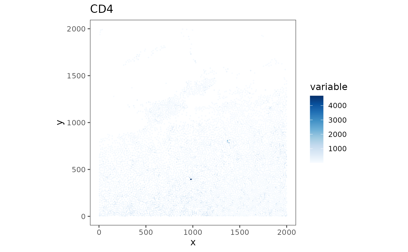
#>
#> $TonsilB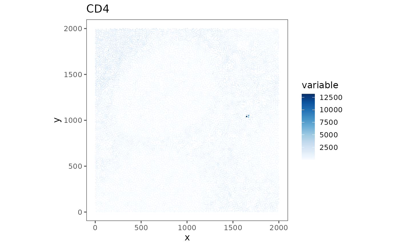
Finally, analyze is a useful debugging tool for the package. Much of SpatialMap’s complexity comes from the grouping structures and the flexibility built in there. Setting analyze = "regions" lets the package functions work in their most simple form.
Review
To review:
-
You can pass
-
"regions"(a special word in SM)
-
- a metadata grouping (e.g., “batch”), or
- an Analysis name (e.g.
"combined") to theanalyzeparameter of most SM functions! This built in flexibility makes it easier to switch modes between single-cell analyses, where spatial coordinates have no consistent meaning, and spatial analyses, where they do.
- an Analysis name (e.g.
Analyses are formal, persistent groupings that allow you to store results in a separate compartment from the original Regions.