Analysis Guide Part III
Unsupervised Clustering with SpatialMap
AnalysisGuide3_Unsupervised_clustering.RmdNavigate vignettes
Reading in data
We will start by reading in our dataset, which had poor quality cells filtered out in part 2 of the analysis guide.
data_file <- "sm_postQC.RDS"

data_dir <- "."
# facil::check_dir is useful if you're running this yourself on code ocean
rw_paths <- facil::check_dir(data_dir)

sm <- readRDS(file.path(rw_paths$read_dir, data_file))
You can recreate this analysis yourself on Code Ocean by attaching the “SpatialMap vignettes” data asset to your capsule and changing
data_dirto/data/spatialmap_vignettes/spatialmap_analysis_guides/
Normalization
Variability in staining intensity and the imprecision in even the best cellular segmentation algorithm makes proper normalization of single cell spatial data crucial. The Normalize function in SpatialMap implements a number of different possible approaches. One approach that has performed well across many studies for us is:
Arcsinh transform the expression data, which transforms the distribution from highly heteroskedastic to approximately normal. This dataset has some biomarkers that have very low values, so we adjust the default function to calculate scale factors.
Center the biomarker expression values for each region on their mean, and then divide by their standard deviation. This puts all the biomarkers in each region on roughly equal footing, and puts all the regions on roughly the same scale.
Similarly scale and center the biomarker expression values of each cell. This can help account for variability across a region in total stain intensity.
scale_factor_function <- function(x) {
  quantile(x + 1, 0.2) * 5
}

sm <- sm %>%

  Normalize(
    method = "asinh",
    scale.factors = scale_factor_function,
    from = "Data",
    to = "NormalizedData"
  ) %>%

  Normalize(
    method = "scale",
    from = "NormalizedData",
    to = "ScaledData"
  ) %>%

  Normalize(
    method = "scale",
    MARGIN = 2,
    from = "ScaledData",
    to = "ScaledData"
  )
#> Normalizing data using method `asinh`
#>
#> Normalizing data using method `scale`
#>
#> Normalizing data using method `scale`
#>
For more information on the different normalization methods available, see
?Normalize
Up until this point, all of our analysis has been on the region level. For clustering, you will usually want to identify phenotypes that are present across your dataset. You can use the Analysis class in SpatialMap to focus future analytical steps on the whole dataset.
sm <- createAnalysis(sm, id = "combined", regions = Regions(sm))
#> New analysis created.
#>  10 Regions
#>  22050 cells
#>  58 common features
#>
#> Added Analysis `combined` to SpatialMap project 'SpatialMap Project'.
#> Setting as active Analysis
#>
Typically, for this first pass of clustering, it is best to focus on markers of broader lineage cell type definitions (e.g. CD45, PanCK, CD3, CD20) rather than markers of cell state that can be expressed across different cell types (e.g. Ki67, which will often pull out a cluster of all proliferating cells), or relatively rarer phenotypes (e.g. CD45RO, LAG3, which can sometimes lump in poorly stained cells with cells that are actually expressing these proteins). You can subsequently do a deeper phenotyping on the cell types you identify in this first round, which the next notebook in this analysis guide will help you perform. There’s no single perfect way to perform this analysis, and you may want to run through a few iterations until you have a clustering that you’re happy with. See the appendix for a list of biomarkers that can be useful if your dataset was acquired using Enable Medicine’s pre-built biomarker panel 1.
An in-depth guide to our recommendations for best practices when performing unsupervised clustering on segmented spatial proteomics data can be found in our user manual–we’d highly recommend checking it out!
This example dataset was acquired outside Enable Medicine’s lab, so we will use a different set of markers for clustering.
unsupervised_markers <- c(
  "CD45", # All immune
  "CD3", "CD4", "CD8", "FoxP3", "CD25", "CD7", # T cells
  "CD20", # B cells
  "CD11b", "CD11c", "CD1a", "CD68", "CD15", "Tryptase", # Myeloid cells
  "CD56", "CD16", # NK and myeloid cells
  "PanCK", # Epithelial cells
  "CD31", "Podoplanin", "Vimentin" # Vascular and stromal cells
)
UMAP
The first step in the clustering workflow in SpatialMap is to create a UMAP embedding. This is useful for visualizing the results of your clustering and normalization approaches. It is generally best to set a random seed prior to running non-deterministic processes such as UMAP and clustering, which will ensure that the results are the same for each of your analyses.
The implementation of UMAP we use in SpatialMap can take advantage of parallel processing to accelerate computation. This means that this step may go faster if you start your workbench session with more than 1 CPU. See the user manual for more detail on how to change this setting when launching a session.
set.seed(59897)
sm <- runUMAP(
  sm,
  data.slot = "ScaledData",
  PCA = T,
  verbose = TRUE,
  n_neighbors = 20,
  min_dist = 0.00001,
  features = unsupervised_markers,
  dims = round(length(unsupervised_markers) * 0.75)
)
#>   By analysis: 'combined'
#>
#> Computing PCA
#>
#> Computing UMAP
#>
#> 16:01:45 UMAP embedding parameters a = 1.933 b = 0.7905
#> 16:01:45 Read 22050 rows and found 15 numeric columns
#> 16:01:46 Building Annoy index with metric = cosine, n_trees = 50
#> 0%   10   20   30   40   50   60   70   80   90   100%
#> [----|----|----|----|----|----|----|----|----|----|
#> **************************************************|
#> 16:01:48 Writing NN index file to temp file /tmp/Rtmp7APXPC/filef4f7c9b129d
#> 16:01:48 Searching Annoy index using 2 threads, search_k = 2000
#> 16:01:52 Annoy recall = 100%
#> 16:01:52 Commencing smooth kNN distance calibration using 2 threads with target n_neighbors = 20
#> 16:01:53 Initializing from normalized Laplacian + noise (using irlba)
#> 16:01:53 Commencing optimization for 200 epochs, with 618098 positive edges
#> 16:02:02 Optimization finished
# As a first pass, try using the first 3/4 of PCs as the inputs for UMAP.
Computing a principal components analysis with
PCA = Tand only using a subset of the components withdims = round(length(unsupervised_markers) * 0.75)focuses your analysis on dominant contributors to variance in your dataset, which are often more biologically relevant. For more information on the parameters you can pass to UMAP, see?runUMAP
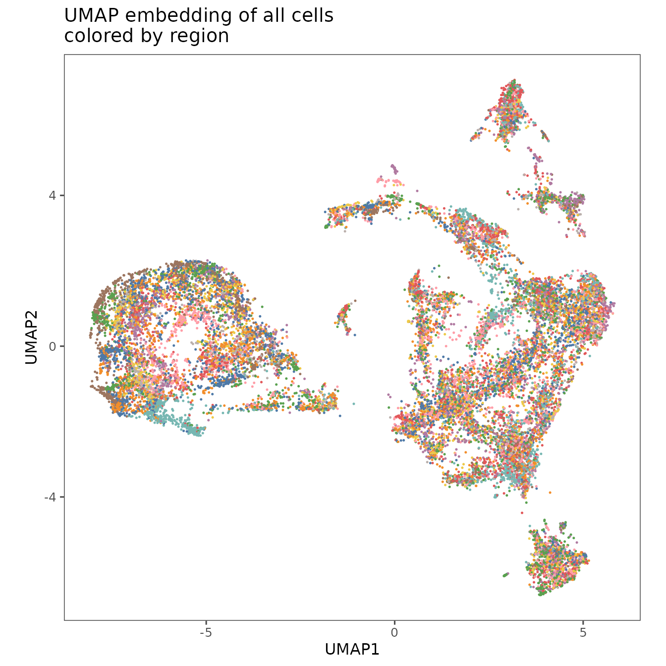
You can visualize the results of your UMAP analysis using plotRepresentation.
plotRepresentation(
  sm,
  "umap",
  what = "region_display_label",
  plot.title = "UMAP embedding of all cells\ncolored by region",
  shuffle = TRUE
) +
  theme(legend.position = "none")
#>   By analysis: 'combined'
#> 
plotRepresentation(
  sm,
  "umap",
  what = "patient_label",
  plot.title = "UMAP embedding of all cells\ncolored by patient",
  shuffle = TRUE
) +
  theme(legend.position = "none")
#>   By analysis: 'combined'
#> 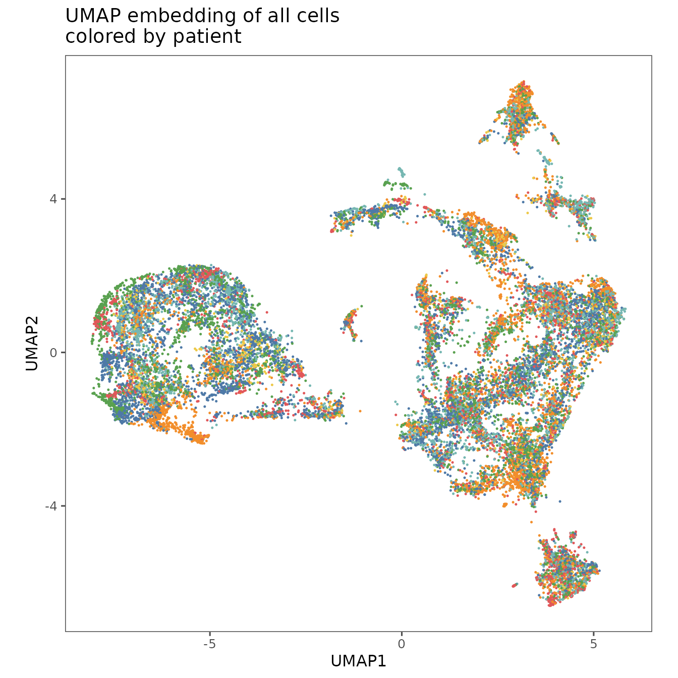
These visualizations show that the patients and regions are all fairly well mixed, which suggests that batch effects are minimal with this normalization approach.
Clustering
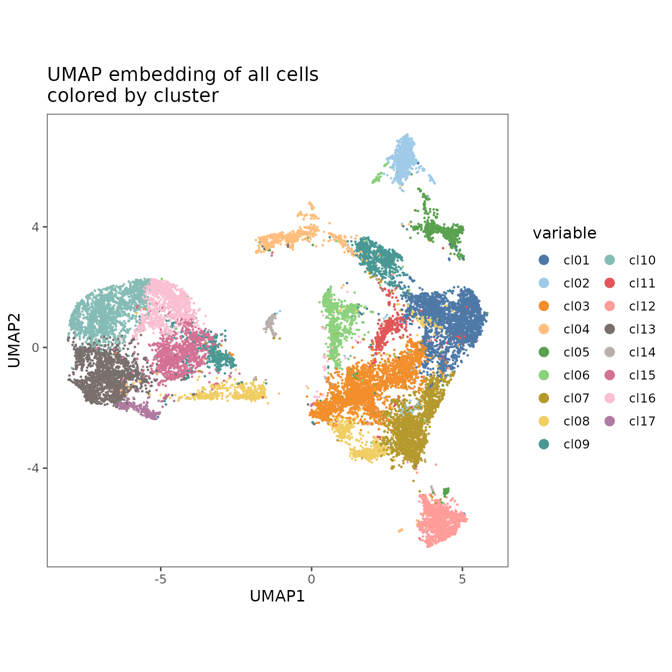
We can now use clusterCells to perform unsupervised clustering. As with UMAP, we set a random seed to ensure that the results will be reproducible.
set.seed(32367)
sm <- clusterCells(sm, method = "leiden", cluster.resolution = 1)
#>   By analysis: 'combined'
#>
We can once again use plotRepresentation to visualize the results overlaid on the UMAP embedding.
plotRepresentation(
  sm,
  "umap",
  what = ".clusters",
  plot.title = "UMAP embedding of all cells\ncolored by cluster",
  shuffle = TRUE
) +
  guides(color = guide_legend(override.aes = list(size = 3),
                              ncol = 2)) # Put legend into two columns with ggplot
#>   By analysis: 'combined'
#> 
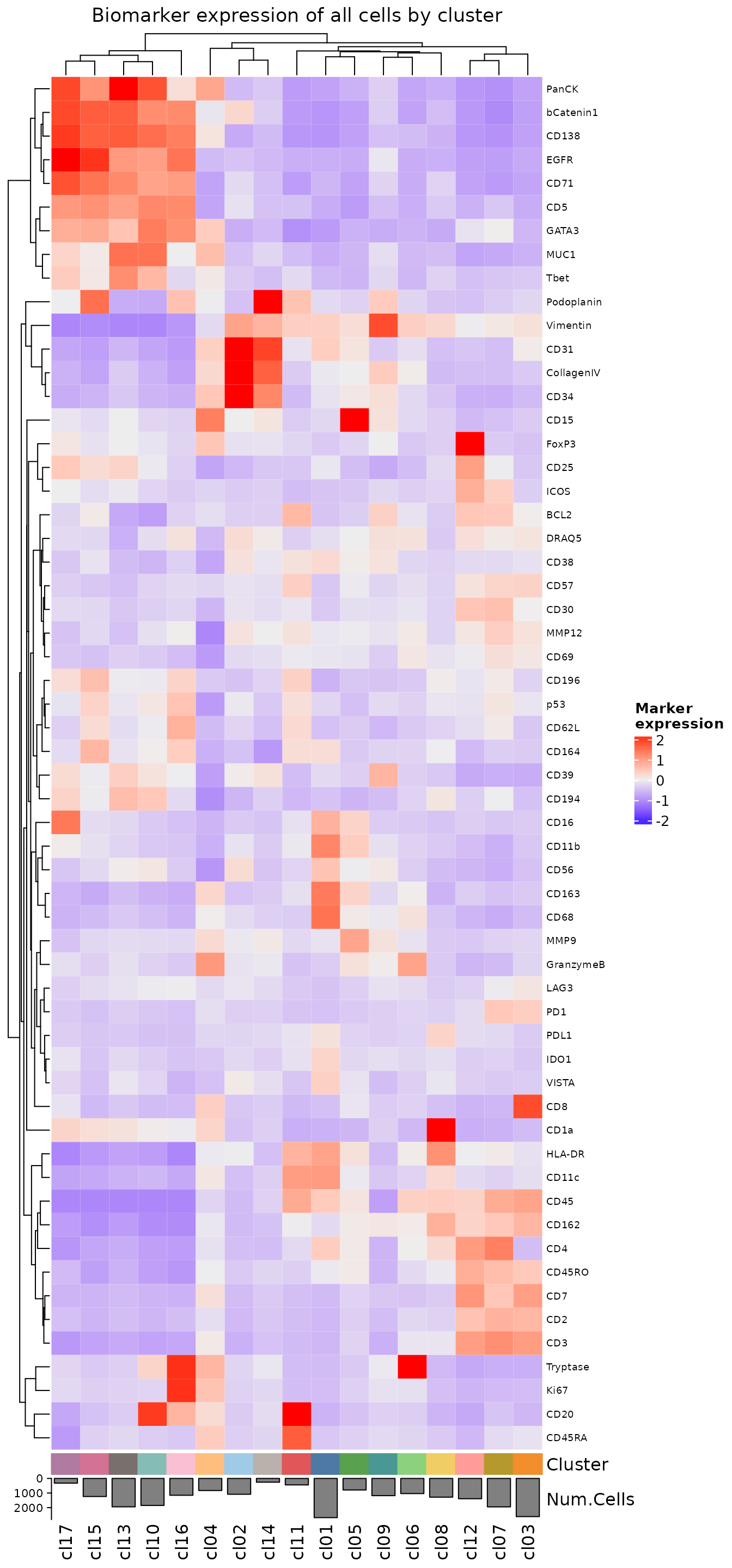
We can also visualize the average biomarker expression profiles using plotExpressionHeatmap.
plotExpressionHeatmap(
  sm,
  data.slot = "ScaledData",
  summary.fun = "median",
  summarize.across = ".clusters",
  scaling = "none",
  column_title = "Biomarker expression of all cells by cluster"
)
#> Plotting expression from slot 'ScaledData'.
#> Scaling = 'none'
#>   By analysis: 'combined'
#> 
It can sometimes be helpful to create a heatmap that only displays a subset of the biomarkers in your panel. Here, we will create a heatmap that shows only the biomarkers used for clustering.
all_markers <- features(sm)

exclude_markers <- all_markers[!(all_markers %in% unsupervised_markers)]

plotExpressionHeatmap(
  sm,
  data.slot = "ScaledData",
  summary.fun = "median",
  summarize.across = ".clusters",
  scaling = "none",
  column_title = "Biomarker expression of all cells by cluster\nonly clustering markers",
  exclude.markers = exclude_markers
)
#> Plotting expression from slot 'ScaledData'.
#> Scaling = 'none'
#>   By analysis: 'combined'
#> 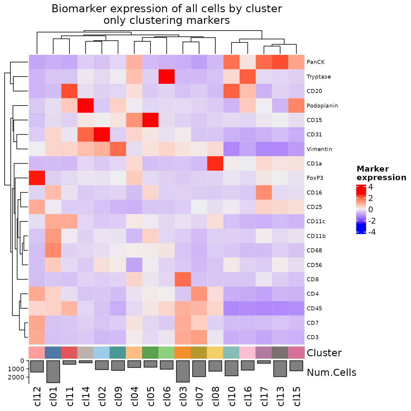
These heatmaps can give a general sense of which cell phenotypes are being captured by this clustering. If there are any phenotypes you would have expected to see that are not being detected, you can try increasing the cluster.resolution in the call to clusterCells. This will encourage the clustering algorithm to identify a larger number of clusters, which can be helpful in detecting low abundance clusters.
It can often be helpful at this stage to push this annotation set to the Portal, so you can generate an overlay in the visualizer. This can help assess the quality of the clustering, and whether the biomarker expressions you are seeing in these heatmaps reflect true expression or imaging/segmentation artifacts. This step is described in further detail in the Tutorial vignette Pushing annotations to the Portal.
uploadCellMetadata(
  object = sm,
  metadata_names = ".clusters",
  uploaded_name = "First pass clustering no labels",
  annotation_description = "The first run of leiden clustering,
  before cell type labels were assigned",
  # Often downstream analysis in the Explorer is
  # less useful before clusters have been given annotations
  create_explorer_output = FALSE
)
As with the QC process, the Insights app can also be a powerful aid to your analysis at this step, and also an excellent resource to other members of your team (or other scientists after publishing the study on the Enable Platform) who would like to look into the work you have done. The function emconnect::upload_image is what allows you to push plots from Workbench to the insights app on the Portal. You can find more information on this process in the Tutorial vignette Pushing plots to the portal.
STUDY_NAME <- projectMetadata(sm)$study_name[[1]]

upload_heatmap <- plotExpressionHeatmap(
  sm,
  data.slot = "ScaledData",
  summary.fun = "median",
  summarize.across = ".clusters",
  scaling = "none",
  column_title = "Biomarker expression of all cells by cluster\nonly clustering markers",
  exclude.markers = exclude_markers
)

upload_image(
  upload_heatmap,
  file.name = "biomarker_heatmap_clustering_markers.png",
  card.title = "Phenotyping from unsupervised clustering on Workbench",
  study_name = STUDY_NAME,
  plot.description = "Biomarker expression heatmap showing median
  expression for clusters from workbench",
  # You may want to try multiple iterations of uploading
  # with different values of height and width to find optimal values
  height = 7,
  width = 7,
  units = "in",
  res = 150
)
See the appendix for more tips on evaluating the cell phenotypes represented by these clusters.
Annotating
Once you have determined which cell phenotype is represented by each cluster, you can add those annotations to your sm object. If you determine that multiple clusters are actually identifying the same phenotype, you can give them the same annotation (e.g. cl15-cl17 below). We have often observed that epithelial PanCK+ phenotypes will split into multiple clusters in a way that appears to represent uneven staining rather than true biological variation.
phenotype_column_name <- "first_round_clustering"

# Assign your clusters to phenotypes here
# Clusters with the same name will be "merged"
cluster.labels <- c(
  cl01 = "Macrophages",
  cl02 = "Dendritic cells",
  cl03 = "CD8+ T cells",
  cl04 = "Other",
  cl05 = "Langerhans cells",
  cl06 = "Mast cells",
  cl07 = "Vimentin+ Stroma",
  cl08 = "Epithelium",
  cl09 = "Epithelium",
  cl10 = "CD8+ T cells",
  cl11 = "CD4+ T cells",
  cl12 = "B cells",
  cl13 = "Langerhans cells",
  cl14 = "T regs",
  cl15 = "Vascular endothelial cells",
  cl16 = "Epithelium",
  cl17 = "Epithelium",
  cl18 = "Lymphatic endothelial cells",
  cl19 = "Epithelium"
)

mapped.vals <- mapValues(as.character(cellMetadata(sm)$.clusters), cluster.labels)
sm <- sm %>% addCellMetadata(mapped.vals, col.names = phenotype_column_name)
Finally, we save our results and proceed to the next part of analysis–subclustering.
Appendix
General clustering guidelines
We have compiled an in-depth guide with our recommendations for best practices for unsupervised clustering of segmented spatial proteomics data, which is available in our user manual.
Clustering marker example
This is often a good set of markers to use for this first round of clustering if your dataset was generating using Enable Medicine’s pre-built biomarker panel 1, but this can depend on the type of tissue you are analyzing.
unsupervised_markers <- c(
  "CD45", # All immune
  "PanCK", "ECad", "EpCAM", # Epithelial lineage
  "CD3e", "CD4", "CD8", "FoxP3", # T cells
  "CD20", # B cells
  "CD14", "CD68", "CD11c", "MPO", # Myeloid cells
  "Vimentin", "aSMA", "CD31", "Podoplanin" # Vascular and stromal cells
)
Identifying which regions have good examples of each cluster
It can often be helpful, when evaluating and annotating a clustering, to look in the Visualizer on the Portal to see exactly which cells have been assigned to each cluster. The code below generates a list of tables for each cluster, showing the number of cells and proportion of each region that is comprised of each of the clusters. This will make it easier to find regions that have a large enough proportion of cells belonging to each cluster to effectively evaluate the cluster assignments.
## retrieve clusters
cell_clusters <- cellMetadata(sm) %>%
  select(region_display_label, .clusters)

## generate cell- and sample-wise cluster counts
cluster_counts <- cell_clusters %>%
  add_count(region_display_label, name = "total_region_cells") %>%
  add_count(region_display_label, .clusters, name = "region_cluster_count") %>%
  distinct()

## compute proportions
cluster_proportions <- cluster_counts %>%
  mutate(region_cluster_frac = region_cluster_count / total_region_cells)

## arrange the result
cluster_abundances_across_regions <- cluster_proportions %>%
  arrange(-region_cluster_frac) %>%
  select(region_display_label,
         .clusters,
         region_cluster_count,
         region_cluster_frac) %>%
  group_split(.clusters)
Resulting tables
cluster_abundances_across_regions
#> <list_of<
#> tbl_df<
#> region_display_label: character
#> .clusters : factor<ceb58>
#> region_cluster_count: integer
#> region_cluster_frac : double
#> >
#> >[17]>
#> [[1]]
#> # A tibble: 10 × 4
#> region_display_label .clusters region_cluster_count region_cluster_frac
#> <chr> <fct> <int> <dbl>
#> 1 41-003.Resp_2 cl01 343 0.168
#> 2 41-005.Pre_1 cl01 163 0.135
#> 3 41-003.Pre_1 cl01 269 0.135
#> 4 07-002.Pre_1 cl01 354 0.134
#> 5 07-004.EOT_1 cl01 294 0.126
#> 6 07-002.EOT_1 cl01 312 0.116
#> 7 41-004.EOT_2 cl01 301 0.115
#> 8 41-001.EOT_2 cl01 292 0.114
#> 9 07-004.Pre_1 cl01 228 0.109
#> 10 41-004.Pre_2 cl01 129 0.0688
#>
#> [[2]]
#> # A tibble: 10 × 4
#> region_display_label .clusters region_cluster_count region_cluster_frac
#> <chr> <fct> <int> <dbl>
#> 1 07-004.EOT_1 cl02 243 0.104
#> 2 07-004.Pre_1 cl02 191 0.0917
#> 3 41-004.EOT_2 cl02 139 0.0530
#> 4 41-003.Pre_1 cl02 92 0.0461
#> 5 41-003.Resp_2 cl02 90 0.0442
#> 6 41-005.Pre_1 cl02 51 0.0422
#> 7 41-001.EOT_2 cl02 106 0.0412
#> 8 41-004.Pre_2 cl02 69 0.0368
#> 9 07-002.Pre_1 cl02 55 0.0208
#> 10 07-002.EOT_1 cl02 49 0.0183
#>
#> [[3]]
#> # A tibble: 10 × 4
#> region_display_label .clusters region_cluster_count region_cluster_frac
#> <chr> <fct> <int> <dbl>
#> 1 07-002.EOT_1 cl03 458 0.171
#> 2 41-004.EOT_2 cl03 402 0.153
#> 3 41-003.Pre_1 cl03 287 0.144
#> 4 07-002.Pre_1 cl03 365 0.138
#> 5 41-003.Resp_2 cl03 259 0.127
#> 6 07-004.EOT_1 cl03 292 0.125
#> 7 41-001.EOT_2 cl03 281 0.109
#> 8 07-004.Pre_1 cl03 132 0.0634
#> 9 41-005.Pre_1 cl03 74 0.0613
#> 10 41-004.Pre_2 cl03 64 0.0342
#>
#> [[4]]
#> # A tibble: 10 × 4
#> region_display_label .clusters region_cluster_count region_cluster_frac
#> <chr> <fct> <int> <dbl>
#> 1 07-002.EOT_1 cl04 148 0.0552
#> 2 41-004.Pre_2 cl04 90 0.0480
#> 3 41-004.EOT_2 cl04 118 0.0450
#> 4 41-001.EOT_2 cl04 115 0.0447
#> 5 07-002.Pre_1 cl04 115 0.0435
#> 6 41-003.Pre_1 cl04 66 0.0331
#> 7 41-003.Resp_2 cl04 52 0.0255
#> 8 41-005.Pre_1 cl04 30 0.0248
#> 9 07-004.Pre_1 cl04 48 0.0230
#> 10 07-004.EOT_1 cl04 46 0.0197
#>
#> [[5]]
#> # A tibble: 10 × 4
#> region_display_label .clusters region_cluster_count region_cluster_frac
#> <chr> <fct> <int> <dbl>
#> 1 41-003.Resp_2 cl05 244 0.120
#> 2 41-001.EOT_2 cl05 155 0.0603
#> 3 41-004.Pre_2 cl05 91 0.0486
#> 4 41-005.Pre_1 cl05 57 0.0472
#> 5 07-004.EOT_1 cl05 65 0.0279
#> 6 41-003.Pre_1 cl05 39 0.0195
#> 7 07-002.Pre_1 cl05 40 0.0151
#> 8 41-004.EOT_2 cl05 39 0.0149
#> 9 07-004.Pre_1 cl05 28 0.0134
#> 10 07-002.EOT_1 cl05 33 0.0123
#>
#> [[6]]
#> # A tibble: 10 × 4
#> region_display_label .clusters region_cluster_count region_cluster_frac
#> <chr> <fct> <int> <dbl>
#> 1 41-004.EOT_2 cl06 199 0.0759
#> 2 07-004.EOT_1 cl06 142 0.0609
#> 3 07-002.Pre_1 cl06 159 0.0602
#> 4 41-005.Pre_1 cl06 66 0.0546
#> 5 41-001.EOT_2 cl06 140 0.0544
#> 6 07-004.Pre_1 cl06 82 0.0394
#> 7 41-003.Pre_1 cl06 68 0.0341
#> 8 41-003.Resp_2 cl06 67 0.0329
#> 9 07-002.EOT_1 cl06 86 0.0321
#> 10 41-004.Pre_2 cl06 28 0.0149
#>
#> [[7]]
#> # A tibble: 10 × 4
#> region_display_label .clusters region_cluster_count region_cluster_frac
#> <chr> <fct> <int> <dbl>
#> 1 07-004.Pre_1 cl07 409 0.196
#> 2 07-004.EOT_1 cl07 262 0.112
#> 3 41-004.Pre_2 cl07 200 0.107
#> 4 41-004.EOT_2 cl07 239 0.0911
#> 5 07-002.Pre_1 cl07 214 0.0810
#> 6 41-003.Resp_2 cl07 163 0.0801
#> 7 41-005.Pre_1 cl07 92 0.0762
#> 8 41-003.Pre_1 cl07 130 0.0651
#> 9 41-001.EOT_2 cl07 139 0.0540
#> 10 07-002.EOT_1 cl07 100 0.0373
#>
#> [[8]]
#> # A tibble: 10 × 4
#> region_display_label .clusters region_cluster_count region_cluster_frac
#> <chr> <fct> <int> <dbl>
#> 1 07-002.Pre_1 cl08 228 0.0863
#> 2 41-001.EOT_2 cl08 212 0.0824
#> 3 07-004.Pre_1 cl08 143 0.0687
#> 4 41-003.Pre_1 cl08 133 0.0666
#> 5 41-005.Pre_1 cl08 79 0.0654
#> 6 41-004.Pre_2 cl08 98 0.0523
#> 7 07-004.EOT_1 cl08 119 0.0510
#> 8 41-004.EOT_2 cl08 106 0.0404
#> 9 07-002.EOT_1 cl08 96 0.0358
#> 10 41-003.Resp_2 cl08 68 0.0334
#>
#> [[9]]
#> # A tibble: 10 × 4
#> region_display_label .clusters region_cluster_count region_cluster_frac
#> <chr> <fct> <int> <dbl>
#> 1 41-005.Pre_1 cl09 96 0.0795
#> 2 07-004.Pre_1 cl09 160 0.0768
#> 3 07-004.EOT_1 cl09 179 0.0767
#> 4 07-002.Pre_1 cl09 167 0.0632
#> 5 41-004.Pre_2 cl09 97 0.0518
#> 6 41-003.Resp_2 cl09 92 0.0452
#> 7 41-001.EOT_2 cl09 107 0.0416
#> 8 41-004.EOT_2 cl09 105 0.0400
#> 9 07-002.EOT_1 cl09 107 0.0399
#> 10 41-003.Pre_1 cl09 69 0.0346
#>
#> [[10]]
#> # A tibble: 9 × 4
#> region_display_label .clusters region_cluster_count region_cluster_frac
#> <chr> <fct> <int> <dbl>
#> 1 41-004.Pre_2 cl10 398 0.212
#> 2 41-003.Pre_1 cl10 258 0.129
#> 3 07-002.EOT_1 cl10 329 0.123
#> 4 41-003.Resp_2 cl10 193 0.0948
#> 5 41-005.Pre_1 cl10 106 0.0877
#> 6 41-001.EOT_2 cl10 213 0.0828
#> 7 07-004.EOT_1 cl10 162 0.0694
#> 8 07-002.Pre_1 cl10 172 0.0651
#> 9 41-004.EOT_2 cl10 20 0.00762
#>
#> [[11]]
#> # A tibble: 10 × 4
#> region_display_label .clusters region_cluster_count region_cluster_frac
#> <chr> <fct> <int> <dbl>
#> 1 07-004.Pre_1 cl11 143 0.0687
#> 2 41-004.EOT_2 cl11 155 0.0591
#> 3 41-003.Resp_2 cl11 32 0.0157
#> 4 41-001.EOT_2 cl11 31 0.0121
#> 5 07-004.EOT_1 cl11 26 0.0111
#> 6 41-003.Pre_1 cl11 14 0.00701
#> 7 41-005.Pre_1 cl11 8 0.00662
#> 8 07-002.Pre_1 cl11 14 0.00530
#> 9 07-002.EOT_1 cl11 12 0.00447
#> 10 41-004.Pre_2 cl11 8 0.00427
#>
#> [[12]]
#> # A tibble: 10 × 4
#> region_display_label .clusters region_cluster_count region_cluster_frac
#> <chr> <fct> <int> <dbl>
#> 1 41-001.EOT_2 cl12 361 0.140
#> 2 41-004.EOT_2 cl12 216 0.0823
#> 3 41-003.Pre_1 cl12 160 0.0802
#> 4 07-004.EOT_1 cl12 163 0.0699
#> 5 41-005.Pre_1 cl12 84 0.0695
#> 6 41-003.Resp_2 cl12 128 0.0629
#> 7 07-002.EOT_1 cl12 123 0.0458
#> 8 07-002.Pre_1 cl12 71 0.0269
#> 9 41-004.Pre_2 cl12 46 0.0245
#> 10 07-004.Pre_1 cl12 39 0.0187
#>
#> [[13]]
#> # A tibble: 10 × 4
#> region_display_label .clusters region_cluster_count region_cluster_frac
#> <chr> <fct> <int> <dbl>
#> 1 07-002.EOT_1 cl13 346 0.129
#> 2 41-004.Pre_2 cl13 236 0.126
#> 3 07-002.Pre_1 cl13 324 0.123
#> 4 41-005.Pre_1 cl13 111 0.0919
#> 5 41-004.EOT_2 cl13 225 0.0858
#> 6 07-004.Pre_1 cl13 174 0.0835
#> 7 41-003.Pre_1 cl13 146 0.0731
#> 8 41-003.Resp_2 cl13 132 0.0648
#> 9 41-001.EOT_2 cl13 144 0.0560
#> 10 07-004.EOT_1 cl13 106 0.0454
#>
#> [[14]]
#> # A tibble: 10 × 4
#> region_display_label .clusters region_cluster_count region_cluster_frac
#> <chr> <fct> <int> <dbl>
#> 1 41-001.EOT_2 cl14 69 0.0268
#> 2 07-004.EOT_1 cl14 57 0.0244
#> 3 41-004.EOT_2 cl14 39 0.0149
#> 4 41-003.Pre_1 cl14 20 0.0100
#> 5 41-005.Pre_1 cl14 9 0.00745
#> 6 07-004.Pre_1 cl14 15 0.00720
#> 7 07-002.EOT_1 cl14 16 0.00596
#> 8 41-003.Resp_2 cl14 11 0.00540
#> 9 07-002.Pre_1 cl14 14 0.00530
#> 10 41-004.Pre_2 cl14 8 0.00427
#>
#> [[15]]
#> # A tibble: 10 × 4
#> region_display_label .clusters region_cluster_count region_cluster_frac
#> <chr> <fct> <int> <dbl>
#> 1 41-005.Pre_1 cl15 156 0.129
#> 2 07-002.EOT_1 cl15 259 0.0965
#> 3 07-002.Pre_1 cl15 225 0.0852
#> 4 07-004.EOT_1 cl15 153 0.0656
#> 5 41-004.Pre_2 cl15 108 0.0576
#> 6 41-004.EOT_2 cl15 141 0.0538
#> 7 41-003.Pre_1 cl15 99 0.0496
#> 8 41-003.Resp_2 cl15 51 0.0250
#> 9 41-001.EOT_2 cl15 39 0.0152
#> 10 07-004.Pre_1 cl15 7 0.00336
#>
#> [[16]]
#> # A tibble: 10 × 4
#> region_display_label .clusters region_cluster_count region_cluster_frac
#> <chr> <fct> <int> <dbl>
#> 1 41-004.Pre_2 cl16 204 0.109
#> 2 41-003.Pre_1 cl16 146 0.0731
#> 3 07-002.EOT_1 cl16 194 0.0723
#> 4 41-004.EOT_2 cl16 179 0.0682
#> 5 41-001.EOT_2 cl16 158 0.0614
#> 6 41-003.Resp_2 cl16 109 0.0535
#> 7 07-002.Pre_1 cl16 111 0.0420
#> 8 41-005.Pre_1 cl16 26 0.0215
#> 9 07-004.EOT_1 cl16 17 0.00729
#> 10 07-004.Pre_1 cl16 9 0.00432
#>
#> [[17]]
#> # A tibble: 6 × 4
#> region_display_label .clusters region_cluster_count region_cluster_frac
#> <chr> <fct> <int> <dbl>
#> 1 07-004.Pre_1 cl17 275 0.132
#> 2 07-002.EOT_1 cl17 15 0.00559
#> 3 07-002.Pre_1 cl17 14 0.00530
#> 4 41-001.EOT_2 cl17 10 0.00389
#> 5 07-004.EOT_1 cl17 7 0.00300
#> 6 41-003.Resp_2 cl17 2 0.000982