Analysis Guide VII
Cohort comparison
AnalysisGuide7_Cohort_comparison.RmdNavigate vignettes
Introduction
Until this point, we have been analyzing our data at the cell and region levels. However, we may be most interested in asking research questions that give us insight into whether cell-level labels differ among patient cohorts defined by their associated clinical metadata (e.g. whether each sample is a primary tumor site or a metastasis, which disease each sample represents, patient outcomes).
For example, we might want to explore whether there are differences in the abundance of cell types or cell-cell interactions for samples across clinical indications.
In this vignette, we will use the statistical approaches in SpatialMap to compare across cohorts the frequencies and spatial relationships of the cell phenotypes defined in the first four Analysis Guide vignettes.
If you have not associated any clinical metadata with your dataset, see the sample traits feature on the portal.
Reading in data
To start, let’s read the data from the previous vignettes.
data_file <- "sm_with_neighborhoods.RDS"

data_dir <- "."
# facil::check_dir is useful if you're running this yourself on code ocean
rw_paths <- facil::check_dir(data_dir)

sm <- readRDS(file.path(rw_paths$read_dir, data_file))
You can recreate this analysis yourself on Code Ocean by attaching the “SpatialMap vignettes” data asset to your capsule and changing
data_dirto/data/spatialmap_vignettes/spatialmap_analysis_guides/
Comparing cell type abundance
The compareCohorts function
To begin, let’s focus on an example research question: do we observe a significant difference in the abundance of cell types (clustering_with_macrophage_subtypes) between patients (patient_label) before and after treatment with Pembrolizumab (time_point)?
To answer this question, we will use the compareCohorts function in SpatialMap, specifying the cell-level label (i.e., feature) we are interested in (feature), the trait in the metadata used to define the cohorts (cohort_colname), and the trait in the metadata that uniquely marks each sample (sample_colname).
Currently, compareCohorts can only handle comparison of two cohorts. As there are more than two levels in time_point, we will specify the two that we would like to compare using select_cohorts.
Note that cell neighborhoods can also be analyzed using
compareCohorts, as well as any categorical cell annotations stored incellMetadata. To see which features and cohort definitions can used with this function, see example code in the Appendix.
cc_results <- compareCohorts(object = sm,
                             feature = "clustering_with_macrophage_subtypes",
                             cohort_colname = "time_point",
                             sample_colname =  "patient_label",
                             select_cohorts = c("Post-treatment", "Pre-treatment")
)
This function counts the cells of each type in the two cohorts, computes their mean proportions (within each sample) across the sample_colname within each cohort, and calculates statistical comparisons between the cohorts for each cell type.
The parameter
select_cohortscan be used to define which cohort will be the “reference” group, and which will be the “comparison” group; the “comparison” group will be the first one in the vector ("Post-treatment"in the example above). Features upregulated in the “reference” group will have negative log fold change values, and features upregulated in the “comparison” group will have positive log fold change values. You can also identify which group is which in the results by looking at the ordering of the column names in the output data frame; the “comparison” cohort will occur first.
cc_results
#>                       cluster   P.Value          P.Value.method       logFC
#> 1                        APCs 0.1422435 Welch Two Sample t-test -1.18047821
#> 2                      T regs 0.1807955 Welch Two Sample t-test  1.66857770
#> 3                     B cells 0.3073100 Welch Two Sample t-test  1.13263833
#> 4                       Other 0.3171864 Welch Two Sample t-test  0.54254651
#> 5                CD8+ T cells 0.3526872 Welch Two Sample t-test  0.37356553
#> 6                  Mast cells 0.3568362 Welch Two Sample t-test  0.54244734
#> 7            Vimentin+ Stroma 0.4904023 Welch Two Sample t-test -0.30261901
#> 8                     M2 > M1 0.5402206 Welch Two Sample t-test  0.30387484
#> 9             Dendritic cells 0.5608024 Welch Two Sample t-test  0.34745739
#> 10 Vascular endothelial cells 0.6322350 Welch Two Sample t-test -0.44936562
#> 11             M1 > M2 CD11c+ 0.6575262 Welch Two Sample t-test  0.17115630
#> 12               CD4+ T cells 0.6594296 Welch Two Sample t-test  0.54332502
#> 13                      PDL1+ 0.6828376 Welch Two Sample t-test  0.41510514
#> 14                 Epithelium 0.8158237 Welch Two Sample t-test -0.10202987
#> 15           Langerhans cells 0.8984526 Welch Two Sample t-test -0.06226006
#> 16                    M1 > M2 0.9170975 Welch Two Sample t-test  0.06910499
#>    mean_proportion_Post-treatment mean_proportion_Pre-treatment mean_proportion
#> 1                     0.004590465                   0.010404376     0.007820416
#> 2                     0.012853031                   0.004043092     0.007958620
#> 3                     0.062099886                   0.028322572     0.043334711
#> 4                     0.027290524                   0.018736527     0.022538304
#> 5                     0.134127541                   0.103529361     0.117128552
#> 6                     0.036747526                   0.025231042     0.030349479
#> 7                     0.046324785                   0.057136129     0.052331087
#> 8                     0.022327792                   0.018087158     0.019971884
#> 9                     0.034087903                   0.026792003     0.030034625
#> 10                    0.032450692                   0.044309464     0.039038899
#> 11                    0.015739151                   0.013978421     0.014760967
#> 12                    0.013665376                   0.009377011     0.011282951
#> 13                    0.024366549                   0.018274055     0.020981830
#> 14                    0.106589713                   0.114400875     0.110929248
#> 15                    0.071213571                   0.074354098     0.072958308
#> 16                    0.009383912                   0.008945019     0.009140083
#>    count_Post-treatment count_Pre-treatment count adj.P.Val adj.P.Val.method
#> 1                    80                 175   255 0.8404155              fdr
#> 2                   181                  66   247 0.8404155              fdr
#> 3                   863                 400  1263 0.8404155              fdr
#> 4                   427                 349   776 0.8404155              fdr
#> 5                  2157                1856  4013 0.8404155              fdr
#> 6                   567                 403   970 0.8404155              fdr
#> 7                   740                1045  1785 0.8404155              fdr
#> 8                   392                 305   697 0.8404155              fdr
#> 9                   537                 458   995 0.8404155              fdr
#> 10                  592                 595  1187 0.8404155              fdr
#> 11                  250                 239   489 0.8404155              fdr
#> 12                  224                 187   411 0.8404155              fdr
#> 13                  322                 294   616 0.8404155              fdr
#> 14                 1611                2055  3666 0.9170975              fdr
#> 15                 1113                1246  2359 0.9170975              fdr
#> 16                  155                 130   285 0.9170975              fdr
Plotting the results
A quick way to represent differential abundance results is in the form of a volcano plot. Here, the volcano plot indicates that CD8+ T cells, lymphatic endothelial cells, and T regs differ the most in abundance between pre- and post-treatment cohorts, with all three cell types more abundant post-treatment than pre-treatment.
plotCohortsVolcano(results = cc_results) +
  ggplot2::labs(title = "Volcano plot of cell type abundance", color = "cell type")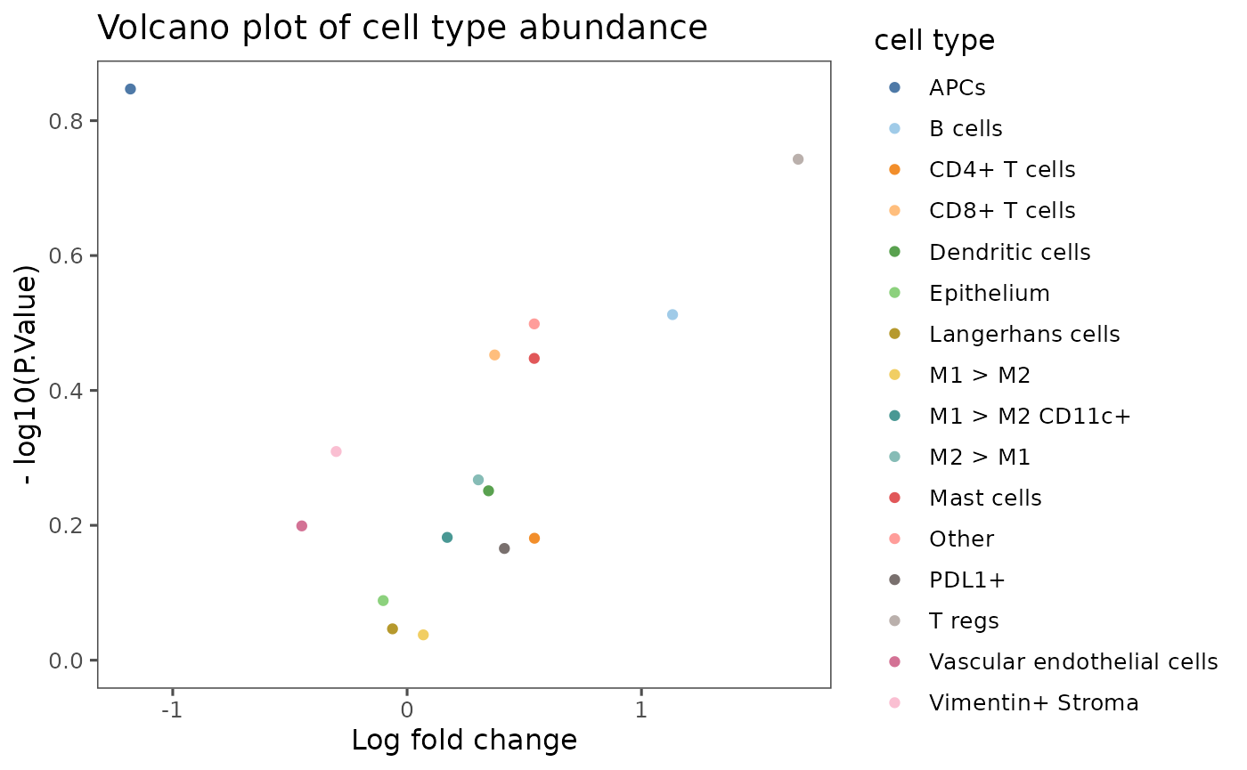
Log2 fold change between cohorts and -log10 of the p-value for the cell type comparison are represented for each feature label (in our case, cell type) as a point in a scatter plot. Points appearing in the top corners of the plot have the largest differential abundance between cohorts, paired with the lowest p-values. Log2 fold change values above 0 are have higher abundance in Cohort 1 (Post-treatment), whereas those below 0 have higher abundance in Cohort 2 (Pre-treatment).
In addition to volcano plots (plotCohortsVolcano()), we can easily use SpatialMap to create plots with plotCellProportions() to summarize the abundance of cell types across defined variables.
Below, we plot the cell proportions across treatment status. As noted from the volcano plot, we see higher abundance of CD8+ T cells, lymphatic endothelial cells, and T regs in the post-treatment cohort.
plotCellProportions(sm,
                    var1 = "clustering_with_macrophage_subtypes",
                    var2 = "time_point",
                    type = "box",
                    select_var2 = c("Post-treatment", "Pre-treatment"))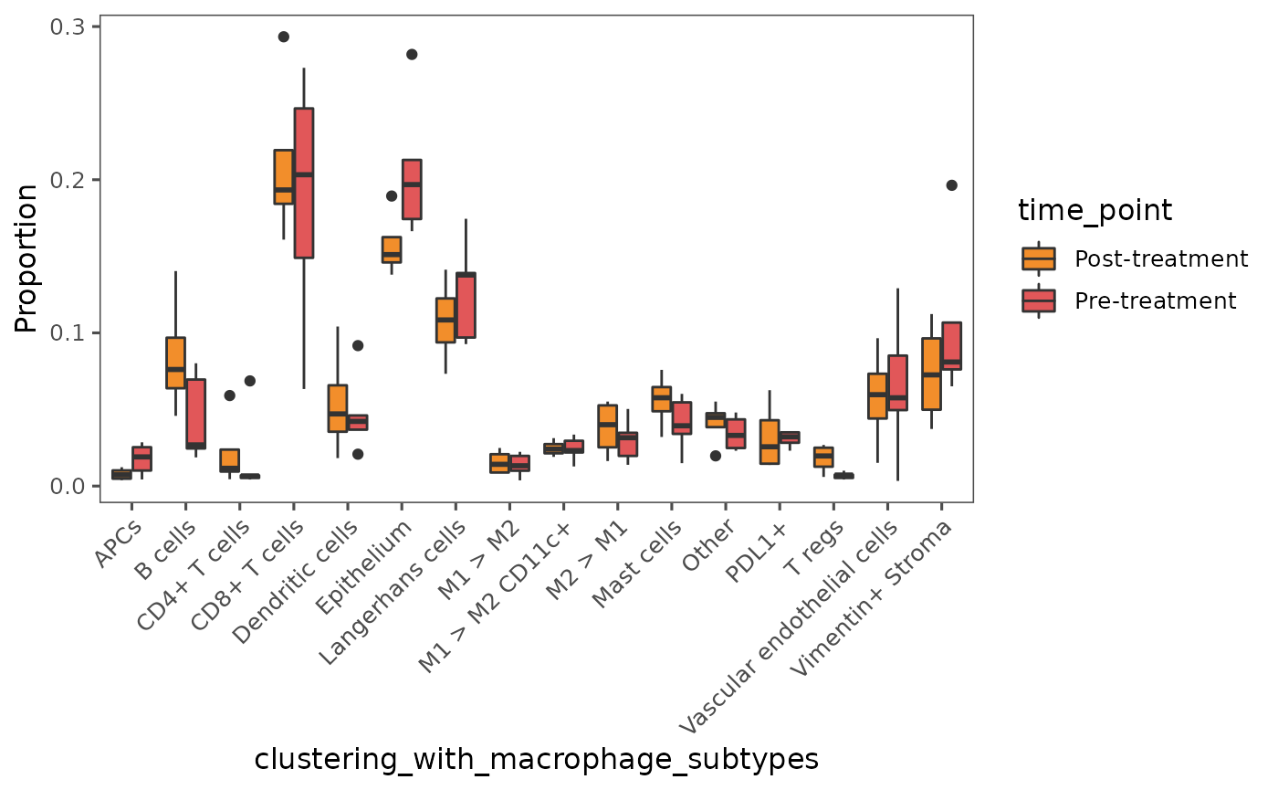
By default,
plotCellProportionsproduces a bar chart. We specifiedtype = "box"to create a boxplot. To learn about additional plot styles available, type?plotCellProportionsinto your console.
In our plots, we can also specify a subset of cell types to display. For example, we can focus on the comparative abundance of T-cell subsets within the data set by defining these as our cell types of interest.
cell_types_of_interest <- c("CD4+ T cells",
                            "CD8+ T cells",
                            "T regs")
When working with plotCellProportions, we can use the argument select_var1 or select_var2 to specify subsets of those respective variables for plotting.
plotCellProportions(sm,
                    var1 = "clustering_with_macrophage_subtypes",
                    var2 = "time_point",
                    type = "box",
                    select_var1 = cell_types_of_interest,
                    select_var2 = c("Pre-treatment", "Post-treatment")
)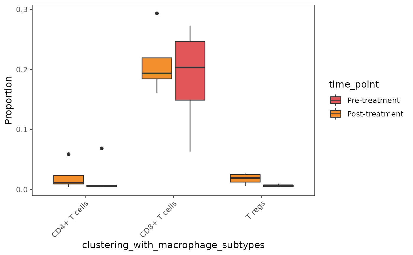
Note that the subset can be defined directly within the call to
plotCellProportions, as we have done withselect_var2, or using a list of the variables of interest can be passed as withselect_var1.
Comparing cell-interactions
The compareAdjacency function
In addition to comparing cell type abundance, we may be interested in understanding whether interactions between different cell types occur with differential frequencies across cohorts. We can use the compareAdjacency function in SpatialMap to compute metrics that will enable such comparisons.
If you haven’t computed pairwise adjacency using the
pairwiseAdjacencyfunction, please see Analysis Guide 5 before proceeding.
# Pulling out region names to define each cohort
cohort1 <- Regions(sm)[projectMetadata(sm)$time_point == "Post-treatment"]
cohort2 <- Regions(sm)[projectMetadata(sm)$time_point == "Pre-treatment"]

# Run the function
ca_out <-
  compareAdjacency(
    object = sm,
    feature = "clustering_with_macrophage_subtypes",
    nn = "spatial_knn_10",
    group.1 = cohort1,
    group.2 = cohort2
  )
Extracting the results
The compareAdjacency function returns a list of data frames with various computations applied. Let’s take a closer look at the third data frame in the list, which contains the results of t-tests comparing the log2-transformed odds ratios of cell interactions between the two cohorts, including both raw and adjusted p.values (by default, adjusted using the "BH" method).
tt_dat <- ca_out$log_odds_t_test %>%
  dplyr::arrange(p.value) %>%
  dplyr::select(feature1, feature2, p.value, everything())

tt_dat %>%
  head(n = 10)
#>        feature1         feature2      p.value statistic diff.in.means
#> t125     T regs          M1 > M2 7.285215e-05 -8.685464     2.0897061
#> t215    M1 > M2           T regs 5.251739e-03 -4.110334     1.7338270
#> t154 Mast cells          M2 > M1 1.073487e-02 -3.955965     0.7603586
#> t208       APCs           T regs 1.091536e-02 -3.663329     1.5056683
#> t169    M2 > M1       Mast cells 1.450743e-02 -3.243108     0.6711033
#> t29      T regs          B cells 1.750151e-02 -3.277836     1.9637347
#> t13      T regs             APCs 2.674297e-02 -2.943144     1.5451601
#> t109     T regs Langerhans cells 2.936872e-02  2.732115    -1.5709982
#> t251      Other Vimentin+ Stroma 4.182842e-02 -2.582012     1.0440971
#> t209    B cells           T regs 4.329697e-02 -2.508510     1.6379141
#>      adjusted.p.value
#> t125       0.01865015
#> t215       0.67222259
#> t154       0.69858313
#> t208       0.69858313
#> t169       0.74278041
#> t29        0.74673115
#> t13        0.93979912
#> t109       0.93979912
#> t251       0.96398648
#> t209       0.96398648
Plotting the results
To make it easier to visualize these results, let’s create our own volcano plot using the ggplot2 package. We will add text labels to the cell pairs with lowest p.value using the ggrepel package.
Under the hood, SpatialMap makes use of the package
ggplot2for plotting, meaning the plots we created above can also be further customized if desired using functions from the package. For more information on how to useggplot2, type?ggplot2} into your console, or see the documentation for theggplot2package.
# Load ggplot2 library
library(ggplot2)

# Make the volcano plot
p1 <- tt_dat %>%
  dplyr::distinct() %>%
  ggplot(aes(x = diff.in.means, y = -log10(p.value))) + # use adjusted.p.value for multiple hypothesis correction
  # Add dashed lines
  geom_vline(xintercept = 0, linetype = "dashed", color = "grey", size = 0.3) +
  geom_hline(yintercept = -log10(0.05), linetype = "dashed", color = "grey", size = 0.3) +
  # Add points
  geom_point() +
  # Add non-overlapping text labels
  ggrepel::geom_text_repel(
    data = dplyr::slice_min(tt_dat, p.value, n = 5), # use adjusted.p.value for multiple hypothesis correction
    aes(label = paste0(feature1, " :: ", feature2)),
    color = "darkblue",
    size = 4,
    min.segment.length = 0.1,
    force = 5
  ) +
  ggthemes::theme_few() +
  theme(aspect.ratio = 1) +
  labs(subtitle = "Volcano plot of cell interactions") +
  lims(y = c(0, NA))

# Print the plot
p1
Based on the volcano plot, a few of the cell type interactions with lowest raw p.value are Vascular endothelial cells :: M1 > M2, M1 > M2 :: Vascular endothelial cells (both more frequent post-treatment), and Epithelium :: PDL1+ APCs (more frequent pre-treatment). Note that, since this analysis typically involves testing an enormous quantity of hypotheses, it’s usually appropriate to use the adjusted p-values.
Conclusion
You have reached the end of the Analysis Guides! To review, we have covered the core functionalities of SpatialMap, including:
- loading your data from ATLAS into a SpatialMap object
- performing QC
- identifying cell phenotypes through unsupervised clustering (and subclustering)
- describing cell interactions
- analyzing spatial neighborhoods
- comparing cell phenotypes across cohorts
As you proceed with your own custom analysis, use these guides as a reference for code snippets and tips. If you find the information provided in the analysis guides doesn’t provide the depth you need to perform your analyses, our Tutorial vignettes offer a deeper dive into the possibilities of analysis with SpatialMap.
Appendix
Selecting features for comparison
Let’s take a closer look at our metadata at both the clinical level and cell level, to better understand what we can compare using compareCohorts and compareAdjacency. We will do this by exploring the column names in projectMetadata and cellMetadata.
Clinical-level features
Clinical metadata are stored at the region-level in projectMetadata:
# Clinical features
clinical_columns <- colnames(projectMetadata(sm))

clinical_columns
#>  [1] "study_id"                     "study_name"
#>  [3] "study_uuid"                   "acquisition_id"
#>  [5] "visual_quality"               "experiment_id"
#>  [7] "experiment_label"             "experiment_uuid"
#>  [9] "assay_metadata"               "assay_name"
#> [11] "assay_description"            "color"
#> [13] "assay_id"                     "axes"
#> [15] "sample_id"                    "region_id"
#> [17] "region_display_label"         "region_uuid"
#> [19] "height"                       "width"
#> [21] "n_levels"                     "n_channels"
#> [23] "n_cycles"                     "time_point"
#> [25] "tissue_type"                  "tissue_subtype"
#> [27] "diagnosis"                    "treatment"
#> [29] "outcome"                      "species"
#> [31] "patient_id"                   "sample_label"
#> [33] "patient_label"                "segmentation_version"
#> [35] "biomarker_expression_version" "Region"
Cell-level metadata
Because our region-level data are also listed in our cell-level metadata, let’s find the columns that cannot be found at the region level:
# Cell-level features
cell_columns <- setdiff(colnames(cellMetadata(sm)),
                        colnames(projectMetadata(sm)))

cell_columns
#>  [1] "cell_id"
#>  [2] "cell.id"
#>  [3] "anno1101_Basic.Cell.Types"
#>  [4] "anno1102_Neighborhood.clustering.based.on.annotation.set.1101"
#>  [5] "anno1970_QC.filters"
#>  [6] "anno1971_First.pass.clustering.no.labels"
#>  [7] "anno2461_Per.region.config.QC.from.Workbench"
#>  [8] "anno2462_per.region.config.clustering.from.workbench"
#>  [9] "cellqc_signal.sum"
#> [10] "cellqc_signal.mean"
#> [11] "cellqc_signal.min"
#> [12] "cellqc_signal.max"
#> [13] "cellqc_signal.median"
#> [14] "cellqc_signal.sd"
#> [15] "cellqc_signal.vars"
#> [16] "cellqc_DNA"
#> [17] "cellqc_cell.size"
#> [18] "cellqc_signal.cv"
#> [19] ".pass_qc"
#> [20] ".qc_result"
#> [21] ".clusters"
#> [22] "first_round_clustering"
#> [23] "clustering_with_macrophage_subtypes"
#> [24] "nh_spatial_knn_10_clustering_with_macrophage_subtypes"
#> [25] "Annotated neighborhoods"
We can explore these features in our dataset by manipulating the data stored in cellMetadata and the dplyr package. Let’s take a look at only the cell-level features by selecting specific columns using dplyr::select. Here we are providing a list of multiple columns to select, and specifying that all of them should be selected using all_of(). For more information on how to use dplyr for analysis (highly recommended!) type ?dplyr::select into your console, or see the documentation for the dplyr package.
# Preview of the cell metadata
cellMetadata(sm) %>%
  dplyr::select(all_of(cell_columns)) %>%
  head()
#>                                     cell_id                             cell.id
#> CITN10Co-88_c001_v001_r001_reg001.1       1 CITN10Co-88_c001_v001_r001_reg001.1
#> CITN10Co-88_c001_v001_r001_reg001.2       2 CITN10Co-88_c001_v001_r001_reg001.2
#> CITN10Co-88_c001_v001_r001_reg001.3       3 CITN10Co-88_c001_v001_r001_reg001.3
#> CITN10Co-88_c001_v001_r001_reg001.4       4 CITN10Co-88_c001_v001_r001_reg001.4
#> CITN10Co-88_c001_v001_r001_reg001.5       5 CITN10Co-88_c001_v001_r001_reg001.5
#> CITN10Co-88_c001_v001_r001_reg001.6       6 CITN10Co-88_c001_v001_r001_reg001.6
#>                                     anno1101_Basic.Cell.Types
#> CITN10Co-88_c001_v001_r001_reg001.1                     PanCK
#> CITN10Co-88_c001_v001_r001_reg001.2                      CD68
#> CITN10Co-88_c001_v001_r001_reg001.3                      CD68
#> CITN10Co-88_c001_v001_r001_reg001.4                     PanCK
#> CITN10Co-88_c001_v001_r001_reg001.5                      CD68
#> CITN10Co-88_c001_v001_r001_reg001.6                       CD8
#>                                     anno1102_Neighborhood.clustering.based.on.annotation.set.1101
#> CITN10Co-88_c001_v001_r001_reg001.1                                                neighborhood_0
#> CITN10Co-88_c001_v001_r001_reg001.2                                                neighborhood_3
#> CITN10Co-88_c001_v001_r001_reg001.3                                                neighborhood_8
#> CITN10Co-88_c001_v001_r001_reg001.4                                                neighborhood_3
#> CITN10Co-88_c001_v001_r001_reg001.5                                                neighborhood_3
#> CITN10Co-88_c001_v001_r001_reg001.6                                                neighborhood_4
#>                                                                  anno1970_QC.filters
#> CITN10Co-88_c001_v001_r001_reg001.1 size_below_threshold, dna_signal_below_threshold
#> CITN10Co-88_c001_v001_r001_reg001.2                       dna_signal_below_threshold
#> CITN10Co-88_c001_v001_r001_reg001.3                                             pass
#> CITN10Co-88_c001_v001_r001_reg001.4                                             pass
#> CITN10Co-88_c001_v001_r001_reg001.5                                             pass
#> CITN10Co-88_c001_v001_r001_reg001.6                                             pass
#>                                     anno1971_First.pass.clustering.no.labels
#> CITN10Co-88_c001_v001_r001_reg001.1                                     cl01
#> CITN10Co-88_c001_v001_r001_reg001.2                                     cl01
#> CITN10Co-88_c001_v001_r001_reg001.3                                     cl01
#> CITN10Co-88_c001_v001_r001_reg001.4                                     cl01
#> CITN10Co-88_c001_v001_r001_reg001.5                                     cl01
#> CITN10Co-88_c001_v001_r001_reg001.6                                     cl03
#>                                     anno2461_Per.region.config.QC.from.Workbench
#> CITN10Co-88_c001_v001_r001_reg001.1                               cell.size, DNA
#> CITN10Co-88_c001_v001_r001_reg001.2                                          DNA
#> CITN10Co-88_c001_v001_r001_reg001.3                                         pass
#> CITN10Co-88_c001_v001_r001_reg001.4                                         pass
#> CITN10Co-88_c001_v001_r001_reg001.5                                         pass
#> CITN10Co-88_c001_v001_r001_reg001.6                                         pass
#>                                     anno2462_per.region.config.clustering.from.workbench
#> CITN10Co-88_c001_v001_r001_reg001.1                                                 cl01
#> CITN10Co-88_c001_v001_r001_reg001.2                                                 cl01
#> CITN10Co-88_c001_v001_r001_reg001.3                                                 cl01
#> CITN10Co-88_c001_v001_r001_reg001.4                                                 cl01
#> CITN10Co-88_c001_v001_r001_reg001.5                                                 cl01
#> CITN10Co-88_c001_v001_r001_reg001.6                                                 cl03
#>                                     cellqc_signal.sum cellqc_signal.mean
#> CITN10Co-88_c001_v001_r001_reg001.1          25330.01           436.7242
#> CITN10Co-88_c001_v001_r001_reg001.2          58453.56          1007.8200
#> CITN10Co-88_c001_v001_r001_reg001.3          46715.99           805.4480
#> CITN10Co-88_c001_v001_r001_reg001.4          35643.20           614.5380
#> CITN10Co-88_c001_v001_r001_reg001.5          41093.25           708.5044
#> CITN10Co-88_c001_v001_r001_reg001.6          51264.24           883.8662
#>                                     cellqc_signal.min cellqc_signal.max
#> CITN10Co-88_c001_v001_r001_reg001.1                 0          4630.336
#> CITN10Co-88_c001_v001_r001_reg001.2                 0          8153.736
#> CITN10Co-88_c001_v001_r001_reg001.3                 0          8893.865
#> CITN10Co-88_c001_v001_r001_reg001.4                 0          5008.797
#> CITN10Co-88_c001_v001_r001_reg001.5                 0         10894.346
#> CITN10Co-88_c001_v001_r001_reg001.6                 0          5085.145
#>                                     cellqc_signal.median cellqc_signal.sd
#> CITN10Co-88_c001_v001_r001_reg001.1             113.9085         876.0841
#> CITN10Co-88_c001_v001_r001_reg001.2             274.9015        1610.3169
#> CITN10Co-88_c001_v001_r001_reg001.3             267.0245        1347.2146
#> CITN10Co-88_c001_v001_r001_reg001.4             197.7965         961.2644
#> CITN10Co-88_c001_v001_r001_reg001.5             238.4820        1537.4162
#> CITN10Co-88_c001_v001_r001_reg001.6             368.7355        1115.7692
#>                                     cellqc_signal.vars cellqc_DNA
#> CITN10Co-88_c001_v001_r001_reg001.1           767523.3   1385.300
#> CITN10Co-88_c001_v001_r001_reg001.2          2593120.5   1123.673
#> CITN10Co-88_c001_v001_r001_reg001.3          1814987.2   2478.791
#> CITN10Co-88_c001_v001_r001_reg001.4           924029.2   1725.944
#> CITN10Co-88_c001_v001_r001_reg001.5          2363648.6   1667.747
#> CITN10Co-88_c001_v001_r001_reg001.6          1244940.9   4446.828
#>                                     cellqc_cell.size cellqc_signal.cv .pass_qc
#> CITN10Co-88_c001_v001_r001_reg001.1              131         2.006035    FALSE
#> CITN10Co-88_c001_v001_r001_reg001.2              178         1.597822    FALSE
#> CITN10Co-88_c001_v001_r001_reg001.3              163         1.672628     TRUE
#> CITN10Co-88_c001_v001_r001_reg001.4              172         1.564207     TRUE
#> CITN10Co-88_c001_v001_r001_reg001.5              306         2.169946     TRUE
#> CITN10Co-88_c001_v001_r001_reg001.6              372         1.262373     TRUE
#>                                         .qc_result .clusters
#> CITN10Co-88_c001_v001_r001_reg001.1 cell.size, DNA      cl01
#> CITN10Co-88_c001_v001_r001_reg001.2            DNA      cl01
#> CITN10Co-88_c001_v001_r001_reg001.3           pass      cl01
#> CITN10Co-88_c001_v001_r001_reg001.4           pass      cl01
#> CITN10Co-88_c001_v001_r001_reg001.5           pass      cl01
#> CITN10Co-88_c001_v001_r001_reg001.6           pass      cl03
#>                                     first_round_clustering
#> CITN10Co-88_c001_v001_r001_reg001.1            Macrophages
#> CITN10Co-88_c001_v001_r001_reg001.2            Macrophages
#> CITN10Co-88_c001_v001_r001_reg001.3            Macrophages
#> CITN10Co-88_c001_v001_r001_reg001.4            Macrophages
#> CITN10Co-88_c001_v001_r001_reg001.5            Macrophages
#> CITN10Co-88_c001_v001_r001_reg001.6           CD8+ T cells
#>                                     clustering_with_macrophage_subtypes
#> CITN10Co-88_c001_v001_r001_reg001.1                             M1 > M2
#> CITN10Co-88_c001_v001_r001_reg001.2                      M1 > M2 CD11c+
#> CITN10Co-88_c001_v001_r001_reg001.3                      M1 > M2 CD11c+
#> CITN10Co-88_c001_v001_r001_reg001.4                             M2 > M1
#> CITN10Co-88_c001_v001_r001_reg001.5                             M1 > M2
#> CITN10Co-88_c001_v001_r001_reg001.6                        CD8+ T cells
#>                                     nh_spatial_knn_10_clustering_with_macrophage_subtypes
#> CITN10Co-88_c001_v001_r001_reg001.1                                        neighborhood_2
#> CITN10Co-88_c001_v001_r001_reg001.2                                        neighborhood_6
#> CITN10Co-88_c001_v001_r001_reg001.3                                        neighborhood_3
#> CITN10Co-88_c001_v001_r001_reg001.4                                        neighborhood_3
#> CITN10Co-88_c001_v001_r001_reg001.5                                        neighborhood_2
#> CITN10Co-88_c001_v001_r001_reg001.6                                        neighborhood_3
#>                                                     Annotated neighborhoods
#> CITN10Co-88_c001_v001_r001_reg001.1                         T cell-dominant
#> CITN10Co-88_c001_v001_r001_reg001.2                                    <NA>
#> CITN10Co-88_c001_v001_r001_reg001.3 Vasculature and perivascular infiltrate
#> CITN10Co-88_c001_v001_r001_reg001.4 Vasculature and perivascular infiltrate
#> CITN10Co-88_c001_v001_r001_reg001.5                         T cell-dominant
#> CITN10Co-88_c001_v001_r001_reg001.6 Vasculature and perivascular infiltrate
To summarize a feature, we can also look at distinct values within a given feature:
cell_types <- cellMetadata(sm) %>%
  dplyr::pull(clustering_with_macrophage_subtypes) %>%
  unique()

cell_types
#>  [1] "M1 > M2"                    "M1 > M2 CD11c+"
#>  [3] "M2 > M1"                    "CD8+ T cells"
#>  [5] "Other"                      "Mast cells"
#>  [7] "Epithelium"                 "Vimentin+ Stroma"
#>  [9] "CD4+ T cells"               "Langerhans cells"
#> [11] "PDL1+"                      "B cells"
#> [13] "Dendritic cells"            "APCs"
#> [15] "T regs"                     "Vascular endothelial cells"
Additional reading
Lianoglou, S., Akridgerunner, & Lun, A. (2015). Limma producing too many significant results. Bioconductor Forum. Retrieved October 24, 2022, from https://support.bioconductor.org/p/67385/
Phipson, B., Sim, C. B., Porrello, E. R., Hewitt, A. W., Powell, J., & Oshlack, A. (2022). propeller: testing for differences in cell type proportions in single cell data. Bioinformatics, 38(20), 4720–4726. https://doi.org/10.1093/bioinformatics/btac582
Quinn, T. P., Erb, I., Gloor, G., Notredame, C., Richardson, M. F., & Crowley, T. M. (2019). A field guide for the compositional analysis of any-omics data. GigaScience, 8(9). https://doi.org/10.1093/gigascience/giz107
Ritchie, M. E., Phipson, B., Wu, D., Hu, Y., Law, C. W., Shi, W., & Smyth, G. K. (2015). Limma powers differential expression analyses for RNA-sequencing and Microarray Studies. Nucleic Acids Research, 43(7). https://doi.org/10.1093/nar/gkv007
Simmons, S. (2022). Cell type composition analysis: comparison of statistical methods. bioRxiv, 2022.02.04.479123. https://doi.org/10.1101/2022.02.04.479123
Weiss, S., Xu, Z. Z., Peddada, S., Amir, A., Bittinger, K., Gonzalez, A., Lozupone, C., Zaneveld, J. R., Vázquez-Baeza, Y., Birmingham, A., Hyde, E. R., & Knight, R. (2017). Normalization and microbial differential abundance strategies depend upon data characteristics. Microbiome, 5(1). https://doi.org/10.1186/s40168-017-0237-y