Tutorial: Advanced spatial analysis
Tutorial_Advanced_spatial.RmdIntroduction
The SpatialMap package has a whole host of tools for performing spatial analyses. This vignette will demonstrate the advanced tools that weren’t mentioned in the Analysis Guide.
We’ll load in the demo dataset sm_skin.
sm <- load_sm_data("skin")Computing graphs
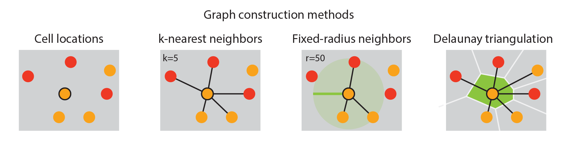
We can compute multiple graphs with SpatialMap: - Fixed-radius nearest neighbors (frNN), which indexes all cells within a fixed distance of the center cell - K nearest neighbors (KNN), which indexes the “K” nearest cells - Shared KNN, which is identical to the KNN, but only includes two-way interactions. - The Delaunay triangulation between cells, which is a subgraph of the KNN with certain special properties.
These methods are called using the method parameter. Except for the Delaunay, methods require either a k parameter or an eps parameter (defining the distance radius for frNN).
sm <- spatialNearestNeighbors(sm, method = "del")
sm <- spatialNearestNeighbors(sm, method = "knn", k = 10)
sm <- spatialNearestNeighbors(sm, method = "snn", k = 10)
sm <- spatialNearestNeighbors(sm, method = "frnn", eps = 50)
To achieve clearer interpretability, you may want to determine how distances in microns convert into distances in pixels for your image. If your object was created using spatialmap_from_db, the projectMetadata slot should contain the information you need for this conversion. This resolution will be given as µm/pixel.
image_res <- projectMetadata(sm) %>%
  dplyr::mutate(image_mpp = purrr::map_dbl(assay_metadata,
                                           ~jsonlite::fromJSON(.x)$image_mpp)) %>%
  dplyr::pull(image_mpp) %>%
  unique()

if (length(image_res) != 1) {
  warning("Pixels will have a different ratio to µm in different images in this dataset.")
}
To convert from a distance in microns to the equivalent distance in pixels, divide your distance in microns by image_res.
This is especially useful for the frnn method, so you can define the radius in microns and then convert to pixels. It is also useful with the del method’s dist_filter argument, which allows you to exclude interactions with cells beyond a certain distance. The Delaunay method’s expansions can sometimes cross gaps in the tissue, which might actually represent genuine biological barriers to communication.
dist_in_microns <- 40
sm <- spatialNearestNeighbors(sm, method = "del", dist_filter = dist_in_microns / image_res)

radius_in_microns <- 20
sm <- spatialNearestNeighbors(sm, method = "frnn", eps = radius_in_microns / image_res)
Side note on neighbors computations
Because spatial nearest neighbors can only be interpreted within a physical context, the spatialNearestNeighbors function above forces activeAnalysis to be regions. Computing spatial neighbors between two different samples wouldn’t have any meaning. The more general function computeNearestNeighbors allows you to compute graphs from coordinate systems that span multiple Regions, such as expression PCAs.
The following lines of code are equivalent:
sm <- spatialNearestNeighbors(sm,
                              method = "del",
                              dist_filter = round(dist_in_microns / image_res))
sm <- computeNearestNeighbors(sm,
                              "spatial_del",
                              method = "del",
                              representation = "spatial",
                              dist_filter = round(dist_in_microns / image_res))
Accessing graphs
Once computed, a nearest neighbor object can easily be accessed and manipulated. Basic accessor methods can be used to view the data:
## Return a list of all NN objects in a SpatialMap analysis
NNs(sm)
#> $Skin1
#> $Skin1$spatial_del
#> Delaunay triangulation object
#>  Median neighbors = 5
#>  4969 cells
#>  igraph: No
#>
#> $Skin1$spatial_knn_10
#> KNN object
#>  10 nearest neighbors
#>  4969 cells
#>  igraph: No
#>
#> $Skin1$spatial_snn_10
#> Shared NN object
#>  Median nearest neighbors = 10
#>  4969 cells
#>  igraph: No
#>
#> $Skin1$spatial_frnn_50
#> Fixed radius NN object
#>  Radius = 50
#>  4969 cells
#>  igraph: No
#>
#> $Skin1$spatial_frnn_53.0503978779841
#> Fixed radius NN object
#>  Radius = 54
#>  4969 cells
#>  igraph: No
#>
#>
#> $Skin2
#> $Skin2$spatial_del
#> Delaunay triangulation object
#>  Median neighbors = 5
#>  4185 cells
#>  igraph: No
#>
#> $Skin2$spatial_knn_10
#> KNN object
#>  10 nearest neighbors
#>  4185 cells
#>  igraph: No
#>
#> $Skin2$spatial_snn_10
#> Shared NN object
#>  Median nearest neighbors = 10
#>  4185 cells
#>  igraph: No
#>
#> $Skin2$spatial_frnn_50
#> Fixed radius NN object
#>  Radius = 50
#>  4185 cells
#>  igraph: No
#>
#> $Skin2$spatial_frnn_53.0503978779841
#> Fixed radius NN object
#>  Radius = 54
#>  4185 cells
#>  igraph: No
#>
#>
#> $Skin3
#> $Skin3$spatial_del
#> Delaunay triangulation object
#>  Median neighbors = 5
#>  3158 cells
#>  igraph: No
#>
#> $Skin3$spatial_knn_10
#> KNN object
#>  10 nearest neighbors
#>  3158 cells
#>  igraph: No
#>
#> $Skin3$spatial_snn_10
#> Shared NN object
#>  Median nearest neighbors = 10
#>  3158 cells
#>  igraph: No
#>
#> $Skin3$spatial_frnn_50
#> Fixed radius NN object
#>  Radius = 50
#>  3158 cells
#>  igraph: No
#>
#> $Skin3$spatial_frnn_53.0503978779841
#> Fixed radius NN object
#>  Radius = 54
#>  3158 cells
#>  igraph: No
#>
#>
#> $Skin4
#> $Skin4$spatial_del
#> Delaunay triangulation object
#>  Median neighbors = 6
#>  5673 cells
#>  igraph: No
#>
#> $Skin4$spatial_knn_10
#> KNN object
#>  10 nearest neighbors
#>  5673 cells
#>  igraph: No
#>
#> $Skin4$spatial_snn_10
#> Shared NN object
#>  Median nearest neighbors = 10
#>  5673 cells
#>  igraph: No
#>
#> $Skin4$spatial_frnn_50
#> Fixed radius NN object
#>  Radius = 50
#>  5673 cells
#>  igraph: No
#>
#> $Skin4$spatial_frnn_53.0503978779841
#> Fixed radius NN object
#>  Radius = 54
#>  5673 cells
#>  igraph: No
#>
#>
#> $Skin5
#> $Skin5$spatial_del
#> Delaunay triangulation object
#>  Median neighbors = 6
#>  3606 cells
#>  igraph: No
#>
#> $Skin5$spatial_knn_10
#> KNN object
#>  10 nearest neighbors
#>  3606 cells
#>  igraph: No
#>
#> $Skin5$spatial_snn_10
#> Shared NN object
#>  Median nearest neighbors = 10
#>  3606 cells
#>  igraph: No
#>
#> $Skin5$spatial_frnn_50
#> Fixed radius NN object
#>  Radius = 50
#>  3606 cells
#>  igraph: No
#>
#> $Skin5$spatial_frnn_53.0503978779841
#> Fixed radius NN object
#>  Radius = 54
#>  3606 cells
#>  igraph: No
#>
#>
#> $Skin6
#> $Skin6$spatial_del
#> Delaunay triangulation object
#>  Median neighbors = 6
#>  3966 cells
#>  igraph: No
#>
#> $Skin6$spatial_knn_10
#> KNN object
#>  10 nearest neighbors
#>  3966 cells
#>  igraph: No
#>
#> $Skin6$spatial_snn_10
#> Shared NN object
#>  Median nearest neighbors = 10
#>  3966 cells
#>  igraph: No
#>
#> $Skin6$spatial_frnn_50
#> Fixed radius NN object
#>  Radius = 50
#>  3966 cells
#>  igraph: No
#>
#> $Skin6$spatial_frnn_53.0503978779841
#> Fixed radius NN object
#>  Radius = 54
#>  3966 cells
#>  igraph: No

## Return a list of NN objects in a Region
reg <- sm[[1]]
NNs(reg)
#> $spatial_del
#> Delaunay triangulation object
#>  Median neighbors = 5
#>  4969 cells
#>  igraph: No
#>
#> $spatial_knn_10
#> KNN object
#>  10 nearest neighbors
#>  4969 cells
#>  igraph: No
#>
#> $spatial_snn_10
#> Shared NN object
#>  Median nearest neighbors = 10
#>  4969 cells
#>  igraph: No
#>
#> $spatial_frnn_50
#> Fixed radius NN object
#>  Radius = 50
#>  4969 cells
#>  igraph: No
#>
#> $spatial_frnn_53.0503978779841
#> Fixed radius NN object
#>  Radius = 54
#>  4969 cells
#>  igraph: No

## Return a single, specific NN object
NNs(reg, "spatial_del")
#> Delaunay triangulation object
#>  Median neighbors = 5
#>  4969 cells
#>  igraph: No

## Return the adjacency list / matrix from an NN object
nn <- NNs(reg, "spatial_del")
head(nn.idx(nn))
#> $Skin1.3055
#> [1]  7 10 26 38 43
#>
#> $Skin1.3060
#> [1] 16 23
#>
#> $Skin1.3063
#> [1] 18 82
#>
#> $Skin1.3065
#> [1] 31 35 60
#>
#> $Skin1.3066
#> [1] 28 58 88
#>
#> $Skin1.3069
#> [1] 29 32 37 55 63

## Return the distances list / matrix from an NN object
head(nn.dist(nn))
#> $Skin1.3055
#> [1] 97.32934 99.32271 85.44004 33.73426 48.37355
#>
#> $Skin1.3060
#> [1] 17.11724 37.64306
#>
#> $Skin1.3063
#> [1] 17.00000 94.04786
#>
#> $Skin1.3065
#> [1] 46.01087 91.18114 55.00000
#>
#> $Skin1.3066
#> [1] 99.46356 98.61541 80.00625
#>
#> $Skin1.3069
#> [1] 76.65507 91.41663 61.74140 71.84010 44.38468

## Add an igraph representation to an NN object
nn <- add_igraph(nn)

## Return the igraph representation from an object
nn.igraph(nn)
#> IGRAPH 163c080 DNW- 4969 26094 --
#> + attr: name (v/c), weight (e/n), distance (e/n)
#> + edges from 163c080 (vertex names):
#>  [1] Skin1.3055->Skin1.3070 Skin1.3055->Skin1.3073 Skin1.3055->Skin1.3100
#>  [4] Skin1.3055->Skin1.3117 Skin1.3055->Skin1.3124 Skin1.3060->Skin1.3083
#>  [7] Skin1.3060->Skin1.3093 Skin1.3063->Skin1.3085 Skin1.3063->Skin1.3175
#> [10] Skin1.3065->Skin1.3107 Skin1.3065->Skin1.3113 Skin1.3065->Skin1.3145
#> [13] Skin1.3066->Skin1.3102 Skin1.3066->Skin1.3143 Skin1.3066->Skin1.3185
#> [16] Skin1.3069->Skin1.3104 Skin1.3069->Skin1.3109 Skin1.3069->Skin1.3116
#> [19] Skin1.3069->Skin1.3138 Skin1.3069->Skin1.3148 Skin1.3070->Skin1.3055
#> [22] Skin1.3070->Skin1.3177 Skin1.3071->Skin1.3101 Skin1.3071->Skin1.3106
#> + ... omitted several edges

## Return the method used to generate the object
nn.method(nn)
#> [1] "del"

## Return any miscellaneous information generated through this object
## The Delaunay object has a good deal of metadata included and stored - other
## methods may have nothing here by default
facil::med(nn.misc(nn))
#> List length 1
#>
#> Names: tri
#> List length 11
#>
#> Names: n, x, y, nt, trlist, cclist...
#> Integer vector,  length:  1
#> Numeric vector,  length:  4969
#> Numeric vector,  length:  4969
#> Integer vector,  length:  1
#> Matrix dim 9908 x 9
#>
#> Matrix dim 9908 x 5
#> $tri
#> $tri$n
#> [1] 4969
#>
#> $tri$x
#> [1]  850 3333 3818 1991 1068  582
#>
#> $tri$y
#> [1] 4085 4085 4084 4083 4080 4078
#>
#> $tri$nt
#> [1] 9908
#>
#> $tri$trlist
#>      i1 i2 i3 j1 j2 j3
#> [1,]  1 43 38  4 12  2
#> [2,] 26 43  1  1  8  6
#> [3,] 38 69 84 13 18  4
#> [4,] 69 38 43  1  9  3
#> [5,] 86 43 48  6 14  9
#> [6,] 43 26 48 11  5  2
#>
#> $tri$cclist
#>             x        y        r   area     ratio
#> [1,] 820.4578 4074.024 31.51522  249.0 0.1559245
#> [2,] 806.3389 4082.092 43.75783 1434.0 0.3369061
#> [3,] 872.6967 4038.507 32.61841  368.5 0.1992114
#> [4,] 839.8605 4037.375 14.95867  251.0 0.4465034
#> [5,] 800.1931 4023.633 32.26584 1059.0 0.4168944
#> [6,] 798.8925 4058.098 31.02853  535.0 0.2566144
Manipulating graphs
Various methods exist within the package - some based off of methods found in the igraph package - to manipulate NN objects.
## Check self-interactions, returning a logical
checkSelfInteractions(nn)
#> [1] FALSE

## Drop self-interactions, if they exist:
dropSelfInteractions(nn)
#> Delaunay triangulation object
#>  Median neighbors = 5
#>  4969 cells
#>  igraph: Yes

## Convert an NN object to `igraph`
NN_to_igraph(nn)
#> IGRAPH f1ecca5 DNW- 4969 26094 --
#> + attr: name (v/c), weight (e/n), distance (e/n)
#> + edges from f1ecca5 (vertex names):
#>  [1] Skin1.3055->Skin1.3070 Skin1.3055->Skin1.3073 Skin1.3055->Skin1.3100
#>  [4] Skin1.3055->Skin1.3117 Skin1.3055->Skin1.3124 Skin1.3060->Skin1.3083
#>  [7] Skin1.3060->Skin1.3093 Skin1.3063->Skin1.3085 Skin1.3063->Skin1.3175
#> [10] Skin1.3065->Skin1.3107 Skin1.3065->Skin1.3113 Skin1.3065->Skin1.3145
#> [13] Skin1.3066->Skin1.3102 Skin1.3066->Skin1.3143 Skin1.3066->Skin1.3185
#> [16] Skin1.3069->Skin1.3104 Skin1.3069->Skin1.3109 Skin1.3069->Skin1.3116
#> [19] Skin1.3069->Skin1.3138 Skin1.3069->Skin1.3148 Skin1.3070->Skin1.3055
#> [22] Skin1.3070->Skin1.3177 Skin1.3071->Skin1.3101 Skin1.3071->Skin1.3106
#> + ... omitted several edges

## Convert the underlying representation of an NN object to a list
knn <- NNs(reg, "spatial_knn_10")
head(nn.idx(knn))
#>            [,1] [,2] [,3] [,4] [,5] [,6] [,7] [,8] [,9] [,10]
#> Skin1.3055   38   43   69   84   26   86   48    7   10    41
#> Skin1.3060   16   23   52   90   62   99   77   11  142    53
#> Skin1.3063   18   82   19  161  106   51  159  148  116   135
#> Skin1.3065   31   60   57   56   35   42  109   25  124    73
#> Skin1.3066   88   58   28    7   33   39  156  153  105   118
#> Skin1.3069   63   37   55   29   44   32  107    9   45    14
knnl <- nn.MatrixToAdjacencyList(NNs(reg, "spatial_knn_10"))
head(nn.dist(knnl))
#> $Skin1.3055
#>  [1]  33.73426  48.37355  62.28965  81.49233  85.44004  85.72631  88.68484
#>  [8]  97.32934  99.32271 109.20165
#>
#> $Skin1.3060
#>  [1]  17.11724  37.64306  50.35871  86.00000 109.07795 125.87692 127.02756
#>  [8] 137.52454 167.86900 170.49633
#>
#> $Skin1.3063
#>  [1]  17.00000  94.04786 175.92328 195.54283 205.97330 222.46348 236.23929
#>  [8] 239.00628 241.64644 251.60286
#>
#> $Skin1.3065
#>  [1]  46.01087  55.00000  61.29437  73.59348  91.18114 107.33592 114.97826
#>  [8] 122.00000 138.17742 141.32233
#>
#> $Skin1.3066
#>  [1]  80.00625  98.61541  99.46356 121.03718 123.76187 170.65755 176.77670
#>  [8] 183.17478 183.33030 190.68561
#>
#> $Skin1.3069
#>  [1]  44.38468  61.74140  71.84010  76.65507  86.92526  91.41663 107.93517
#>  [8] 108.04166 124.04032 124.25780