SpatialMap Quickstart: Introduction and Feature Demo
Quickstart_guide.RmdNavigate vignettes
library(facil)
library(emconnect)
library(SpatialMap)
library(dplyr)
library(patchwork)
library(ggplot2)
library(ggthemes)
SpatialMap Intro
Importing data
SpatialMap is a suite of tools for exploratory spatial biology data analysis built on some convenient data abstractions.
To get started quickly, let’s load a toy SpatialMap (sm_tonsil) object containing CODEX data.
sm_tonsil <- load_sm_data("tonsil")Object / class basics
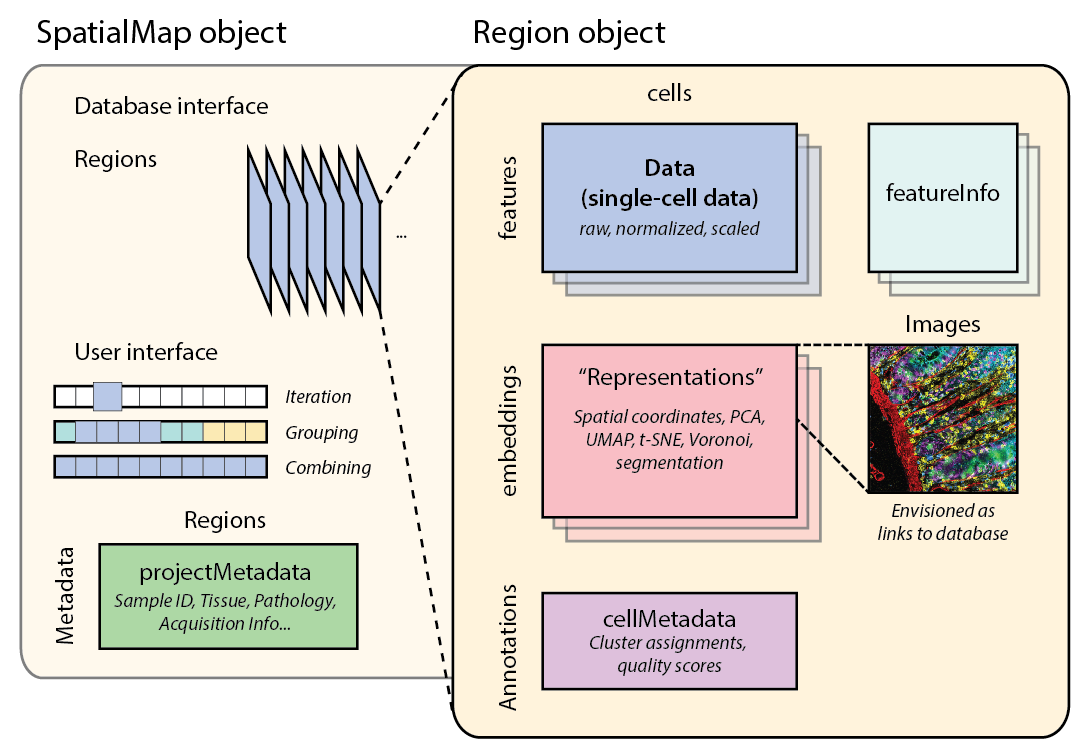
SpatialMap Schematic
The SpatialMap package is powered by abstractions (classes) that help represent and work with key aspects of spatial biology data. Those abstractions are: - SpatialMap - Region - Analysis - Representation - NN (nearest neighbors)
The package provides an interface such that users should primarily only need to interact with the main SpatialMap object. However, documentation for each of the other classes is provided, and more information about a particular object can be found using the str() method on the console.
SpatialMap
A SpatialMap object is a container that holds annotated spatial biology data. An object can be consist of multiple individual samples or acquisitions, which are called Regions. Regions can be combined as an Analysis. The SpatialMap object itself contains project information such as sample metadata, analysis settings, and feature information.
sm_tonsil
#> SpatialMap object
#> Active analysis:  regions
#> +  16,504 total cells
#> +  16 features
#> +  2 Regions:
#>   - TonsilA
#>   - TonsilB
projectMetadata(sm_tonsil) %>% head()
#>             color width n_channels height           projection_visualizer_uuid
#> TonsilA grayscale  9408          4   9072 96e6af5a-f612-4f97-a294-c580dcd41915
#> TonsilB grayscale  9408          4   9072 f0b41218-209e-4946-9a1d-1fb7fb3e7a0d
#>         sample_label n_levels assay_id n_cycles
#> TonsilA  EnableShare        5        1        8
#> TonsilB EnableShare2        5        1        8
#>                   base_image_visualizer_uuid experiment_label axes
#> TonsilA 728d42b7-77ea-4319-a48a-7f7340bf182d      enableshare TCYX
#> TonsilB 2007da53-7ede-492e-84b6-f2d2ab32a09d     enableshare2 TCYX
#>                                    assay_metadata assay_description
#> TonsilA {"image_mpp": 0.377, "num_amp_cycles": 0}
#> TonsilB {"image_mpp": 0.377, "num_amp_cycles": 0}
#>         experiment_id visual_quality assay_name region_display_label
#> TonsilA           164           true      CODEX          EnableShare
#> TonsilB           355           true      CODEX         EnableShare2
#>         biomarker_expression_version segmentation_version  Region coverslip_id
#> TonsilA                            1                    1 TonsilA          164
#> TonsilB                            1                    1 TonsilB          164
#>            study_name
#> TonsilA Enable Tonsil
#> TonsilB Enable Tonsil
cells(sm_tonsil) %>% head()
#> [1] "TonsilA.125182" "TonsilA.125238" "TonsilA.125254" "TonsilA.125325"
#> [5] "TonsilA.125326" "TonsilA.125608"
Regions(sm_tonsil)
#> [1] "TonsilA" "TonsilB"
showsettings(sm_tonsil)
#>                    Parameter                    Value
#> 1                      cores                        1
#> 2                   parallel                   future
#> 3         future.initialized                    FALSE
#> 4              show.progress                    FALSE
#> 5                    Rstudio                     TRUE
#> 6                python.path                     none
#> 7         python.environment            spatialmap_py
#> 8              python.method               reticulate
#> 9                   platform                     unix
#> 10              local.images                    FALSE
#> 11                filtration                     soft
#> 12             normalization                      log
#> 13             max_cell.size                     1600
#> 14             min_cell.size                      100
#> 15            max_signal.sum                   125000
#> 16            min_signal.sum                     5000
#> 17             max_signal.cv                        4
#> 18             min_signal.cv                        1
#> 19 max_normalized.signal.sum                       70
#> 20 min_normalized.signal.sum                       10
#> 21                   max_DNA                    10000
#> 22                   min_DNA                      500
#> 23           max_num.markers                       40
#> 24           min_num.markers                        2
#> 25                max_dist.n                      300
#> 26           max_dist.smooth                      100
#> 27        exclude_partitions
#> 28        SpatialMap.version 0.5.20-->Repaired_0.5.25
As an exercise, we can add to the projectMetadata using straightforward R conventions
new.pm <- projectMetadata(sm_tonsil)
new.pm[["sample_label"]] <- c("sample1", "sample2")

projectMetadata(sm_tonsil) <- new.pm
Region
A Region holds the expression data, cell coordinates, cell metadata, spatial analyses, and more. It is very similar to an anndata object in Python or a SingleCellExperiment object in R.
cellMetadata(sm_tonsil) %>% head()
#> cell_id cell.id anno316_some_categories anno916_Leiden_v1
#> TonsilA.125182 125182 TonsilA.125182 yay Cluster 2
#> TonsilA.125238 125238 TonsilA.125238 nay Cluster 2
#> TonsilA.125254 125254 TonsilA.125254 yay Cluster 1
#> TonsilA.125325 125325 TonsilA.125325 yay Cluster 1
#> TonsilA.125326 125326 TonsilA.125326 nay Cluster 6
#> TonsilA.125608 125608 TonsilA.125608 nay Cluster 1
#> anno248_test_subset_annotation_324
#> TonsilA.125182 p
#> TonsilA.125238 u
#> TonsilA.125254 t
#> TonsilA.125325 t
#> TonsilA.125326 b
#> TonsilA.125608 y
#> anno1189_uqc_test10_letters_qc_assoc anno1149_uqc_test10_letters
#> TonsilA.125182 b b
#> TonsilA.125238 b b
#> TonsilA.125254 b b
#> TonsilA.125325 c c
#> TonsilA.125326 c c
#> TonsilA.125608 b b
#> anno1133_uqc_test03_letters anno247_test_letters_324
#> TonsilA.125182 l p
#> TonsilA.125238 k u
#> TonsilA.125254 z t
#> TonsilA.125325 f t
#> TonsilA.125326 f b
#> TonsilA.125608 m y
#> anno1190_uqc_test10_letters_qc_assoc_postfilt
#> TonsilA.125182 <NA>
#> TonsilA.125238 <NA>
#> TonsilA.125254 b
#> TonsilA.125325 <NA>
#> TonsilA.125326 <NA>
#> TonsilA.125608 <NA>
#> anno253_Hierarchy.1 anno1797_uqc_test10_letters_221213
#> TonsilA.125182 not Th c
#> TonsilA.125238 not Th b
#> TonsilA.125254 Epithelial Cells b
#> TonsilA.125325 Epithelial Cells b
#> TonsilA.125326 Endothelial Cells b
#> TonsilA.125608 Epithelial Cells b
#> anno254_Neighborhood.clustering.based.on.annotation.set.253
#> TonsilA.125182 neighborhood_2
#> TonsilA.125238 neighborhood_2
#> TonsilA.125254 neighborhood_0
#> TonsilA.125325 neighborhood_0
#> TonsilA.125326 neighborhood_2
#> TonsilA.125608 neighborhood_0
#> anno1145_uqc_test08_letters anno1143_uqc_test08_letters Region
#> TonsilA.125182 l l TonsilA
#> TonsilA.125238 k k TonsilA
#> TonsilA.125254 z z TonsilA
#> TonsilA.125325 f f TonsilA
#> TonsilA.125326 f f TonsilA
#> TonsilA.125608 m m TonsilA
#> color width n_channels height
#> TonsilA.125182 grayscale 9408 4 9072
#> TonsilA.125238 grayscale 9408 4 9072
#> TonsilA.125254 grayscale 9408 4 9072
#> TonsilA.125325 grayscale 9408 4 9072
#> TonsilA.125326 grayscale 9408 4 9072
#> TonsilA.125608 grayscale 9408 4 9072
#> projection_visualizer_uuid sample_label n_levels
#> TonsilA.125182 96e6af5a-f612-4f97-a294-c580dcd41915 EnableShare 5
#> TonsilA.125238 96e6af5a-f612-4f97-a294-c580dcd41915 EnableShare 5
#> TonsilA.125254 96e6af5a-f612-4f97-a294-c580dcd41915 EnableShare 5
#> TonsilA.125325 96e6af5a-f612-4f97-a294-c580dcd41915 EnableShare 5
#> TonsilA.125326 96e6af5a-f612-4f97-a294-c580dcd41915 EnableShare 5
#> TonsilA.125608 96e6af5a-f612-4f97-a294-c580dcd41915 EnableShare 5
#> assay_id n_cycles base_image_visualizer_uuid
#> TonsilA.125182 1 8 728d42b7-77ea-4319-a48a-7f7340bf182d
#> TonsilA.125238 1 8 728d42b7-77ea-4319-a48a-7f7340bf182d
#> TonsilA.125254 1 8 728d42b7-77ea-4319-a48a-7f7340bf182d
#> TonsilA.125325 1 8 728d42b7-77ea-4319-a48a-7f7340bf182d
#> TonsilA.125326 1 8 728d42b7-77ea-4319-a48a-7f7340bf182d
#> TonsilA.125608 1 8 728d42b7-77ea-4319-a48a-7f7340bf182d
#> experiment_label segmentation_visualizer_uuid axes
#> TonsilA.125182 enableshare 9d6258e3-1532-40fb-9503-0831f8661358 TCYX
#> TonsilA.125238 enableshare 9d6258e3-1532-40fb-9503-0831f8661358 TCYX
#> TonsilA.125254 enableshare 9d6258e3-1532-40fb-9503-0831f8661358 TCYX
#> TonsilA.125325 enableshare 9d6258e3-1532-40fb-9503-0831f8661358 TCYX
#> TonsilA.125326 enableshare 9d6258e3-1532-40fb-9503-0831f8661358 TCYX
#> TonsilA.125608 enableshare 9d6258e3-1532-40fb-9503-0831f8661358 TCYX
#> assay_metadata assay_description
#> TonsilA.125182 {"image_mpp": 0.377, "num_amp_cycles": 0}
#> TonsilA.125238 {"image_mpp": 0.377, "num_amp_cycles": 0}
#> TonsilA.125254 {"image_mpp": 0.377, "num_amp_cycles": 0}
#> TonsilA.125325 {"image_mpp": 0.377, "num_amp_cycles": 0}
#> TonsilA.125326 {"image_mpp": 0.377, "num_amp_cycles": 0}
#> TonsilA.125608 {"image_mpp": 0.377, "num_amp_cycles": 0}
#> experiment_id visual_quality assay_name region_display_label
#> TonsilA.125182 164 true CODEX EnableShare
#> TonsilA.125238 164 true CODEX EnableShare
#> TonsilA.125254 164 true CODEX EnableShare
#> TonsilA.125325 164 true CODEX EnableShare
#> TonsilA.125326 164 true CODEX EnableShare
#> TonsilA.125608 164 true CODEX EnableShare
#> biomarker_expression_version segmentation_version study_name
#> TonsilA.125182 1 1 Enable Tonsil
#> TonsilA.125238 1 1 Enable Tonsil
#> TonsilA.125254 1 1 Enable Tonsil
#> TonsilA.125325 1 1 Enable Tonsil
#> TonsilA.125326 1 1 Enable Tonsil
#> TonsilA.125608 1 1 Enable Tonsil
featureInfo(sm_tonsil[[1]])
#> features
#> CD3e CD3e
#> CD21 CD21
#> CD68 CD68
#> Actin Actin
#> CD45RO CD45RO
#> HisH3p HisH3p
#> PanCK PanCK
#> Ki67 Ki67
#> CD11c CD11c
#> ECad ECad
#> CD4 CD4
#> CD31 CD31
#> Podoplanin Podoplanin
#> CD107a CD107a
#> CD20 CD20
#> CD8 CD8
# It's sometimes useful to annotate cells with sample-level metadata. We can do this with a quick function call.
# > This is done by default when pulling data from ATLAS
sm_tonsil <- mergeProjectMetadata(sm_tonsil)
cellMetadata(sm_tonsil) %>% head()
#> cell_id cell.id anno316_some_categories anno916_Leiden_v1
#> TonsilA.125182 125182 TonsilA.125182 yay Cluster 2
#> TonsilA.125238 125238 TonsilA.125238 nay Cluster 2
#> TonsilA.125254 125254 TonsilA.125254 yay Cluster 1
#> TonsilA.125325 125325 TonsilA.125325 yay Cluster 1
#> TonsilA.125326 125326 TonsilA.125326 nay Cluster 6
#> TonsilA.125608 125608 TonsilA.125608 nay Cluster 1
#> anno248_test_subset_annotation_324
#> TonsilA.125182 p
#> TonsilA.125238 u
#> TonsilA.125254 t
#> TonsilA.125325 t
#> TonsilA.125326 b
#> TonsilA.125608 y
#> anno1189_uqc_test10_letters_qc_assoc anno1149_uqc_test10_letters
#> TonsilA.125182 b b
#> TonsilA.125238 b b
#> TonsilA.125254 b b
#> TonsilA.125325 c c
#> TonsilA.125326 c c
#> TonsilA.125608 b b
#> anno1133_uqc_test03_letters anno247_test_letters_324
#> TonsilA.125182 l p
#> TonsilA.125238 k u
#> TonsilA.125254 z t
#> TonsilA.125325 f t
#> TonsilA.125326 f b
#> TonsilA.125608 m y
#> anno1190_uqc_test10_letters_qc_assoc_postfilt
#> TonsilA.125182 <NA>
#> TonsilA.125238 <NA>
#> TonsilA.125254 b
#> TonsilA.125325 <NA>
#> TonsilA.125326 <NA>
#> TonsilA.125608 <NA>
#> anno253_Hierarchy.1 anno1797_uqc_test10_letters_221213
#> TonsilA.125182 not Th c
#> TonsilA.125238 not Th b
#> TonsilA.125254 Epithelial Cells b
#> TonsilA.125325 Epithelial Cells b
#> TonsilA.125326 Endothelial Cells b
#> TonsilA.125608 Epithelial Cells b
#> anno254_Neighborhood.clustering.based.on.annotation.set.253
#> TonsilA.125182 neighborhood_2
#> TonsilA.125238 neighborhood_2
#> TonsilA.125254 neighborhood_0
#> TonsilA.125325 neighborhood_0
#> TonsilA.125326 neighborhood_2
#> TonsilA.125608 neighborhood_0
#> anno1145_uqc_test08_letters anno1143_uqc_test08_letters Region
#> TonsilA.125182 l l TonsilA
#> TonsilA.125238 k k TonsilA
#> TonsilA.125254 z z TonsilA
#> TonsilA.125325 f f TonsilA
#> TonsilA.125326 f f TonsilA
#> TonsilA.125608 m m TonsilA
#> color width n_channels height
#> TonsilA.125182 grayscale 9408 4 9072
#> TonsilA.125238 grayscale 9408 4 9072
#> TonsilA.125254 grayscale 9408 4 9072
#> TonsilA.125325 grayscale 9408 4 9072
#> TonsilA.125326 grayscale 9408 4 9072
#> TonsilA.125608 grayscale 9408 4 9072
#> projection_visualizer_uuid sample_label n_levels
#> TonsilA.125182 96e6af5a-f612-4f97-a294-c580dcd41915 EnableShare 5
#> TonsilA.125238 96e6af5a-f612-4f97-a294-c580dcd41915 EnableShare 5
#> TonsilA.125254 96e6af5a-f612-4f97-a294-c580dcd41915 EnableShare 5
#> TonsilA.125325 96e6af5a-f612-4f97-a294-c580dcd41915 EnableShare 5
#> TonsilA.125326 96e6af5a-f612-4f97-a294-c580dcd41915 EnableShare 5
#> TonsilA.125608 96e6af5a-f612-4f97-a294-c580dcd41915 EnableShare 5
#> assay_id n_cycles base_image_visualizer_uuid
#> TonsilA.125182 1 8 728d42b7-77ea-4319-a48a-7f7340bf182d
#> TonsilA.125238 1 8 728d42b7-77ea-4319-a48a-7f7340bf182d
#> TonsilA.125254 1 8 728d42b7-77ea-4319-a48a-7f7340bf182d
#> TonsilA.125325 1 8 728d42b7-77ea-4319-a48a-7f7340bf182d
#> TonsilA.125326 1 8 728d42b7-77ea-4319-a48a-7f7340bf182d
#> TonsilA.125608 1 8 728d42b7-77ea-4319-a48a-7f7340bf182d
#> experiment_label segmentation_visualizer_uuid axes
#> TonsilA.125182 enableshare 9d6258e3-1532-40fb-9503-0831f8661358 TCYX
#> TonsilA.125238 enableshare 9d6258e3-1532-40fb-9503-0831f8661358 TCYX
#> TonsilA.125254 enableshare 9d6258e3-1532-40fb-9503-0831f8661358 TCYX
#> TonsilA.125325 enableshare 9d6258e3-1532-40fb-9503-0831f8661358 TCYX
#> TonsilA.125326 enableshare 9d6258e3-1532-40fb-9503-0831f8661358 TCYX
#> TonsilA.125608 enableshare 9d6258e3-1532-40fb-9503-0831f8661358 TCYX
#> assay_metadata assay_description
#> TonsilA.125182 {"image_mpp": 0.377, "num_amp_cycles": 0}
#> TonsilA.125238 {"image_mpp": 0.377, "num_amp_cycles": 0}
#> TonsilA.125254 {"image_mpp": 0.377, "num_amp_cycles": 0}
#> TonsilA.125325 {"image_mpp": 0.377, "num_amp_cycles": 0}
#> TonsilA.125326 {"image_mpp": 0.377, "num_amp_cycles": 0}
#> TonsilA.125608 {"image_mpp": 0.377, "num_amp_cycles": 0}
#> experiment_id visual_quality assay_name region_display_label
#> TonsilA.125182 164 true CODEX EnableShare
#> TonsilA.125238 164 true CODEX EnableShare
#> TonsilA.125254 164 true CODEX EnableShare
#> TonsilA.125325 164 true CODEX EnableShare
#> TonsilA.125326 164 true CODEX EnableShare
#> TonsilA.125608 164 true CODEX EnableShare
#> biomarker_expression_version segmentation_version study_name
#> TonsilA.125182 1 1 Enable Tonsil
#> TonsilA.125238 1 1 Enable Tonsil
#> TonsilA.125254 1 1 Enable Tonsil
#> TonsilA.125325 1 1 Enable Tonsil
#> TonsilA.125326 1 1 Enable Tonsil
#> TonsilA.125608 1 1 Enable Tonsil
#> coverslip_id
#> TonsilA.125182 164
#> TonsilA.125238 164
#> TonsilA.125254 164
#> TonsilA.125325 164
#> TonsilA.125326 164
#> TonsilA.125608 164Regions can contain Representations, which can be accessed or modified with methods that “get” or “set”. By default, each Region will have a spatial representation, since it must be initialized with X/Y coordinates.
# Save the Region to its own object for now

reg <- sm_tonsil[[1]]

Representations(reg)
#> $spatial
#> Representation object 'spatial'
#>  Dimensions: 'x', 'y'
#>  5810 cells
Representations(reg, "spatial")
#> Representation object 'spatial'
#>  Dimensions: 'x', 'y'
#>  5810 cells
We can plot different features over that spatial information easily.
p1 <- plotRepresentation(reg, "spatial", what = "panck", trim = c(0, .95))
p2 <- plotRepresentation(reg, "spatial", what = "cd8", trim = c(0, .95))
p1 + p2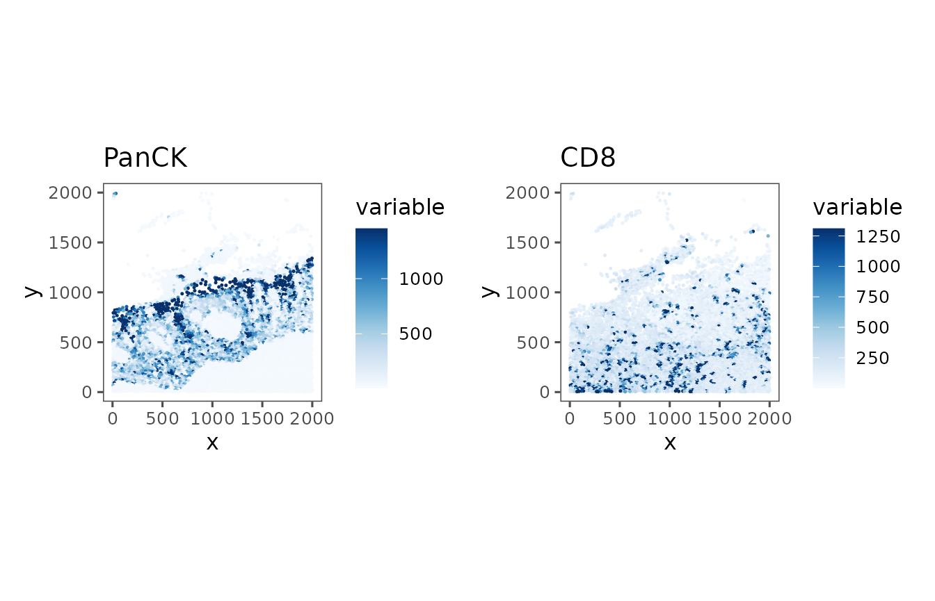
Basic Operations
SpatialMap and Region objects can be subsetted, often using base R syntax, such as [ and [[. We can also use special “setter” methods, such as the features<- function, to subset the features. In this case, features not included in the markers.i.like vector will be dropped. Careful though, as those markers can’t be retrieved from the object.
# Subset SpatialMaps
subset.sm_tonsil <- sm_tonsil[1]

# Subset Region cells
reg.subset <- sm_tonsil[[1]][1:4]

# Subset features
features(reg.subset)
#>  [1] "CD3e"       "CD21"       "CD68"       "Actin"      "CD45RO"
#>  [6] "HisH3p"     "PanCK"      "Ki67"       "CD11c"      "ECad"
#> [11] "CD4"        "CD31"       "Podoplanin" "CD107a"     "CD20"
#> [16] "CD8"

markers.i.like <- c("PanCK", "CD11c", "CD20", "CD8", "Ki67")
features(reg.subset) <- markers.i.like

features(reg.subset)
#> [1] "PanCK" "CD11c" "CD20"  "CD8"   "Ki67"
Creating your own functions
Central to SpatialMap is the idea that the Regions that comprise the object can be modified either as individual samples or in combination. The .smapply() is a powerful function, analagous to R’s apply, that allows users to write their own functions on the SpatialMap object.
Below, we write an anonymous function that subsets each Region to a specific x-y range.
small_tonsil <- .smapply(object = sm_tonsil, function(r) {

  ## Retreive spatial embeddings from Region 'r'
  emb <- embeddings(r, "spatial")

  ## Take the desired subset from the top corner
  my.subset <- emb[, "x"] < 1000 & inv(emb[, "y"]) < 1000

  ## Check that some cells remain (otherwise things could break)
  if (sum(my.subset) < 2) {
    stop("Subset is empty")
  }

  ## Subset Region r and return
  r[my.subset]
})

dim(reg)
#>    cells features
#>     5810       16
dim(small_tonsil[[1]])
#>    cells features
#>      371       16
Data Quality Control and Filtering
Next, we will run functions to calculate basic QC metrics and pass cells through QC filters. The results can be visualized using special plotting functions.
dna <- "DAPI"
sm_tonsil <- sm_tonsil %>%
  QCMetrics(DNA = dna) %>%
  FilterCodex()
#> Calculating quality control metrics...
#>
#> Filtering cells...
#>

qc.list <- plotQCSummary(sm_tonsil, group.variable = "sample_label")
wrap_plots(qc.list)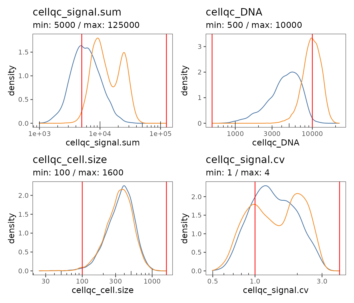
It may be apparent that the QC thresholds used were not perfect. We can easily modify them by updating the object settings, and re-running the QC and Filter commands.
Filter results are stored in cellMetadata, and can be plotted using plotFilteredCells, which is simply a special case of the plotRepresentation function.
showsettings(sm_tonsil)
#>                    Parameter                    Value
#> 1                      cores                        1
#> 2                   parallel                   future
#> 3         future.initialized                    FALSE
#> 4              show.progress                    FALSE
#> 5                    Rstudio                     TRUE
#> 6                python.path                     none
#> 7         python.environment            spatialmap_py
#> 8              python.method               reticulate
#> 9                   platform                     unix
#> 10              local.images                    FALSE
#> 11                filtration                     soft
#> 12             normalization                      log
#> 13             max_cell.size                     1600
#> 14             min_cell.size                      100
#> 15            max_signal.sum                   125000
#> 16            min_signal.sum                     5000
#> 17             max_signal.cv                        4
#> 18             min_signal.cv                        1
#> 19 max_normalized.signal.sum                       70
#> 20 min_normalized.signal.sum                       10
#> 21                   max_DNA                    10000
#> 22                   min_DNA                      500
#> 23           max_num.markers                       40
#> 24           min_num.markers                        2
#> 25                max_dist.n                      300
#> 26           max_dist.smooth                      100
#> 27        exclude_partitions
#> 28        SpatialMap.version 0.5.20-->Repaired_0.5.25
new.settings <- c(
  min_signal.cv = 0.75,
  max_signal.cv = 3.5,
  max_DNA = 20000,
  min_DNA = 250,
  min_signal.sum = 2500,
  max_signal.sum = 100000
)
settings(sm_tonsil, names(new.settings)) <- new.settings

sm_tonsil <- sm_tonsil %>%
  QCMetrics(DNA = dna) %>%
  FilterCodex()
#> Calculating quality control metrics...
#>
#> Filtering cells...
#>

new.fs.list <- plotFilterSummary(sm_tonsil, group.variable = "Region")
wrap_plots(new.fs.list)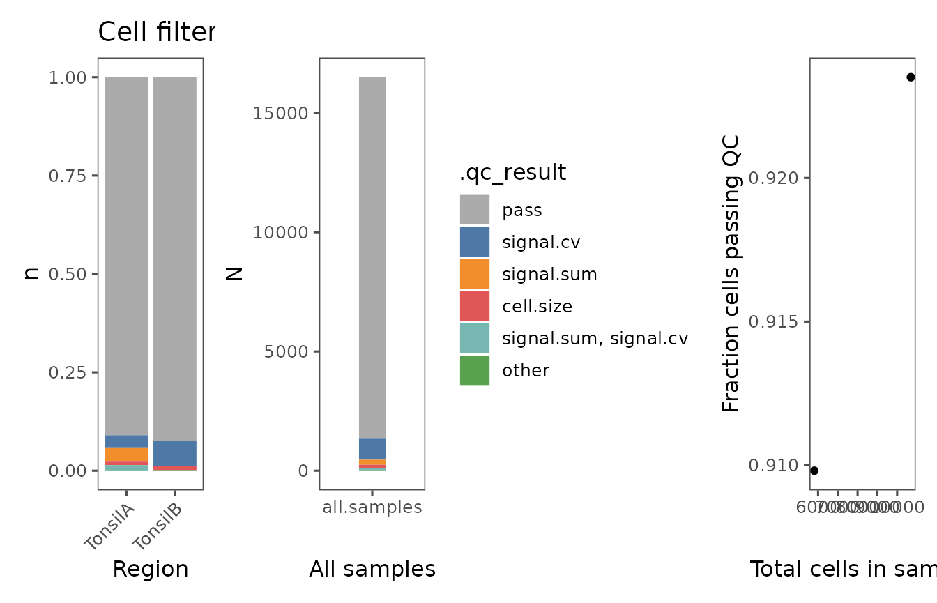
filter.plots <- plotFilteredCells(sm_tonsil)
filter.plots[[1]]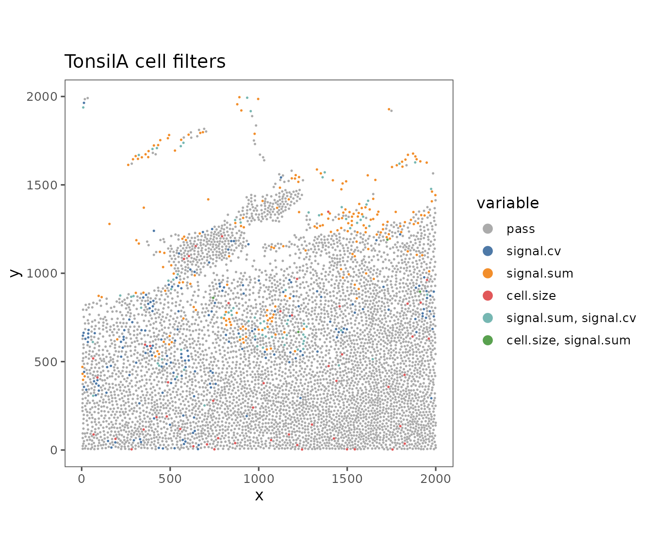
Finally, we may wish to label the filtered cells, or actually remove them entirely from our analysis. The filter function provides a parameter to choose. Note that the removed cells are not preserved anywhere after this step!
sm_tonsil <- FilterCodex(sm_tonsil, remove.filtered.cells = T)Data Normalization and Scaling
SpatialMap implements a select list of scaling and normalization functions curated for spatial proteomics data. Some simple transformations - arcsin transform and robust scaling - are shown below, and users are encouraged to explore the full suite in the Normalize documentation in (?Normalize) in order to find the workflows that best account for batch effects and experiments in their data.
sm_tonsil <- sm_tonsil %>%
  Normalize(method = "asinh", from = "Data", to = "NormalizedData") %>%
  Normalize(method = "scale", from = "NormalizedData", to = "ScaledData")
#> Normalizing data using method `asinh`
#>
#> Normalizing data using method `scale`
#>

featureInfo(sm_tonsil[[1]])
#>              features     0%      10%      20%      30%      40%      50%
#> CD3e             CD3e 13.600  31.7162  35.9138  39.5297  44.1938  49.6145
#> CD21             CD21 57.529 266.8636 339.8682 414.3092 496.8962 605.8785
#> CD68             CD68 43.103 167.8457 191.2824 212.5469 233.0440 259.7695
#> Actin           Actin 19.737  36.5922  39.7528  41.9627  43.8038  45.6465
#> CD45RO         CD45RO 19.584 150.2757 174.6478 196.1867 218.5066 242.2745
#> HisH3p         HisH3p  9.064  48.1388  54.7516  60.1876  65.4418  70.6130
#> PanCK           PanCK  8.109  28.6548  32.7278  37.4576  45.3874  64.8410
#> Ki67             Ki67  3.420  92.9732 119.7084 141.2547 164.7920 195.4330
#> CD11c           CD11c 34.033  82.7721  92.9756 101.8474 110.9640 120.0590
#> ECad             ECad  0.794 137.4073 191.1620 243.4006 293.1336 358.0260
#> CD4               CD4 14.184  50.2858  59.9098  70.1698  81.9488  96.2305
#> CD31             CD31  8.864  31.7347  35.4242  38.5848  41.4254  44.4345
#> Podoplanin Podoplanin  2.376 111.0212 151.6054 199.5184 326.0710 560.9920
#> CD107a         CD107a 26.656  91.2956 125.0510 155.6178 190.9350 225.7370
#> CD20             CD20 22.632 135.6811 268.5706 391.3278 504.6348 612.6625
#> CD8               CD8  0.568  68.9498  97.0338 120.0068 140.4384 162.9525
#>                  60%       70%       80%       90%      100%
#> CD3e         58.7494   75.7193  112.4684  206.1743  1022.907
#> CD21        753.1586  967.7830 1287.6744 1934.0145 15034.270
#> CD68        290.6922  327.3372  385.2952  511.9733 10383.041
#> Actin        47.5920   49.9096   52.9030   57.7335   129.109
#> CD45RO      271.2812  310.7763  362.5008  473.4737  1925.049
#> HisH3p       76.7472   83.9486   95.2082  117.8481  8850.312
#> PanCK       178.2786  339.3262  532.5656  914.7127  7299.914
#> Ki67        237.3502  292.4716  419.2380  996.3913 22920.352
#> CD11c       131.1460  145.3691  167.6772  211.4985  1189.828
#> ECad        440.6974  600.2093  908.2984 1550.6641  6958.132
#> CD4         115.0546  143.9397  191.7948  287.8391  4679.053
#> CD31         48.5814   54.2942   65.1392   95.7470   875.383
#> Podoplanin 1048.1634 1894.0597 3400.1404 5627.5859 29556.791
#> CD107a      263.8120  305.9724  357.9064  443.3744  2948.113
#> CD20        716.9250  826.6439  942.0000 1100.5661  5771.062
#> CD8         193.4120  234.7125  311.4080  649.5986 12148.939
#>            arcsinh_scale_factors
#> CD3e                     179.569
#> CD21                    1699.341
#> CD68                     956.412
#> Actin                    198.764
#> CD45RO                   873.239
#> HisH3p                   273.758
#> PanCK                    163.639
#> Ki67                     598.542
#> CD11c                    464.878
#> ECad                     955.810
#> CD4                      299.549
#> CD31                     177.121
#> Podoplanin               758.027
#> CD107a                   625.255
#> CD20                    1342.853
#> CD8                      485.169

m1 <- "CD8"
par(mfrow = c(1, 3))
r1 <- sm_tonsil[[1]]
hist(Data(r1, "Data")[m1, ])
hist(Data(r1, "NormalizedData")[m1, ])
hist(Data(r1, "ScaledData")[m1, ])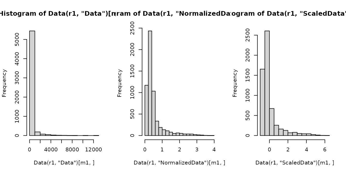
Clustering and Dimensionality Reduction
The Analysis Class
An Analysis is a group of Regions. When an Analysis is active, SpatialMap functions will automatically combine the relevant Region data and operate on the combined data. Otherwise, SpatialMap functions will operate on each Region separately. This logic is all handled through the .smapply() function, which we first discussed above.
Analyses can contain their own Representation objects (for example, PC representations or UMAPs), nearest neighbor graphs, cells, and features.
Here, we activate a new analysis containing both of our Regions in order to run unsupervised clustering on our entire expression data.
sm_tonsil <- createAnalysis(sm_tonsil, id = "combined", regions = Regions(sm_tonsil))
#> New analysis created.
#>  2 Regions
#>  16504 cells
#>  16 common features
#>
#> Added Analysis `combined` to SpatialMap project 'SpatialMap Project'.
#> Setting as active Analysis
#>

sm_tonsil <-
  runUMAP(sm_tonsil,
    data.slot = "ScaledData",
    PCA = TRUE,
    dims = 8,
    n_neighbors = 50,
    verbose = TRUE
  )
#>   By analysis: 'combined'
#>
#> Computing PCA
#>
#> Computing UMAP
#>
#> 16:04:19 UMAP embedding parameters a = 0.9922 b = 1.112
#> 16:04:19 Read 16504 rows and found 8 numeric columns
#> 16:04:20 Building Annoy index with metric = cosine, n_trees = 50
#> 0%   10   20   30   40   50   60   70   80   90   100%
#> [----|----|----|----|----|----|----|----|----|----|
#> **************************************************|
#> 16:04:22 Writing NN index file to temp file /tmp/RtmpHX1Hgq/file106f664b164d
#> 16:04:22 Searching Annoy index using 2 threads, search_k = 5000
#> 16:04:27 Annoy recall = 100%
#> 16:04:28 Commencing smooth kNN distance calibration using 2 threads with target n_neighbors = 50
#> 16:04:29 Initializing from normalized Laplacian + noise (using irlba)
#> 16:04:30 Commencing optimization for 200 epochs, with 1070580 positive edges
#> 16:04:38 Optimization finished

sm_tonsil <- clusterCells(sm_tonsil, method = "leiden")
#>   By analysis: 'combined'
#>
Plotting Representations
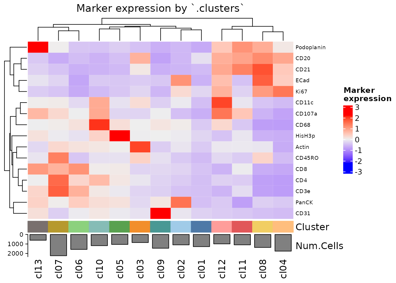
Our UMAP and PCA results can be plotted with the same code as the spatial plots: plotRepresentation(). We can also now plot a summarized heatmap of expression values across clusters.
plotExpressionHeatmap(sm_tonsil, data.slot = "ScaledData", summarize.across = ".clusters", scaling = "none")
#> Plotting expression from slot 'ScaledData'.
#> Scaling = 'none'
#>   By analysis: 'combined'
#> 
pu1 <- plotRepresentation(sm_tonsil, "umap", ".clusters")
#>   By analysis: 'combined'
#>
pu2 <- plotRepresentation(sm_tonsil, "umap", "Region")
#>   By analysis: 'combined'
#>
pu1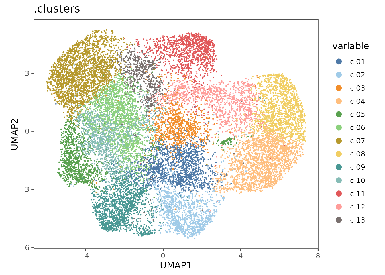
pu2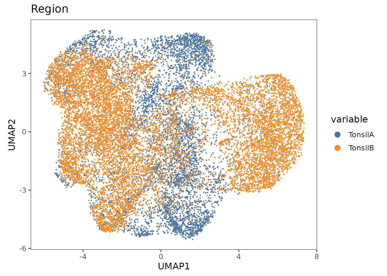
Another common use here is to plot marker expression in the reduced dimensions:
ue1 <- plotRepresentation(sm_tonsil, "umap", "panck", data.slot = "ScaledData")
#>   By analysis: 'combined'
#>
ue2 <- plotRepresentation(sm_tonsil, "umap", "cd8", data.slot = "ScaledData")
#>   By analysis: 'combined'
#>
ue1 + ue2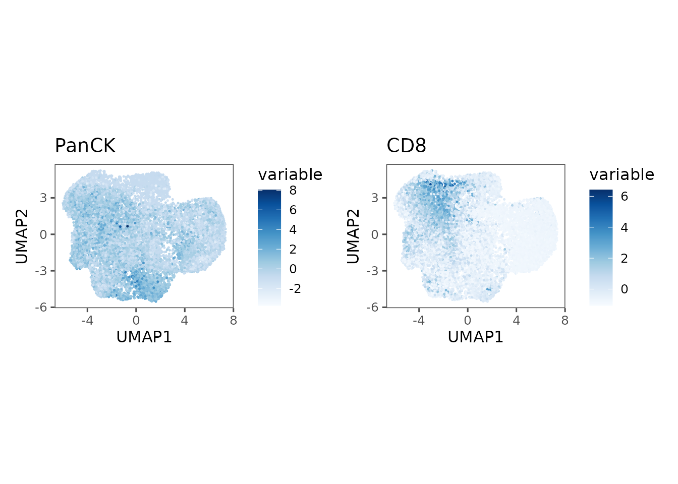
Handling Metadata
Having viewed our expression values by cluster, we might want to annotate them manually. We can use base R to construct a named vector mapping cluster labels to their manual annotations. Then, SpatialMap provides a helper function to map the automatic values to the new ones. Finally, we can add those values to the object in the cellMetadata slot using addCellMetadata()
# Renaming clusters
cluster.labels <- c(
  cl01 = "B Cell",
  cl02 = "T Cell"
)

old.labels <- cellMetadata(sm_tonsil)$.clusters
new.labels <- mapValues(old.labels, cluster.labels)
#> Warning: mapping returned 13926 NA values
sm_tonsil <- addCellMetadata(sm_tonsil, metadata = new.labels, col.names = "Cell.type")
Spatial Analysis
Of course, the most interesting insights from CODEX or other spatial data should be from the spatial information. Here, we demo two methods for spatial analysis. First, pairwise adjacency, which computes how much more likely two cell groups are to interact in space than you would expect by chance (taking into account the graph structure and cell group proportions of a sample).
Statistical analysis of cell neighborhoods in the different samples
activeAnalysis(sm_tonsil) <- "regions"
sm_tonsil <- spatialNearestNeighbors(sm_tonsil, representation = "spatial", method = "knn", k = 5)
sm_tonsil <- pairwiseAdjacency(sm_tonsil, nn = "spatial_knn_5", feature = ".clusters")
pa.plots <- list()
pa.plots[["enrichment"]] <- plotPairwiseAdjacency(
  sm_tonsil,
  nn = "spatial_knn_5",
  feature = ".clusters",
  what = "log10.padj.enrichment",
  cluster_rows = F,
  cluster_columns = F
)
pa.plots[["depletion"]] <- plotPairwiseAdjacency(
  sm_tonsil,
  nn = "spatial_knn_5",
  feature = ".clusters",
  what = "log10.padj.depletion",
  cluster_rows = F,
  cluster_columns = F
)
We can plot those results:
pa.plots$enrichment[[1]]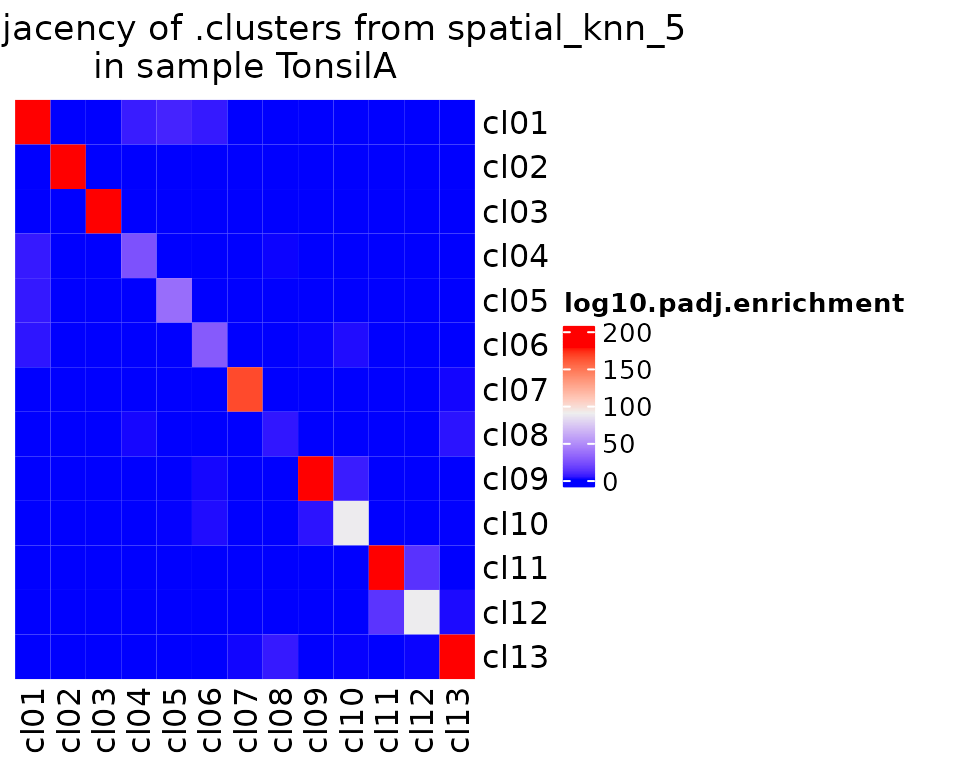
pa.plots$depletion[[1]]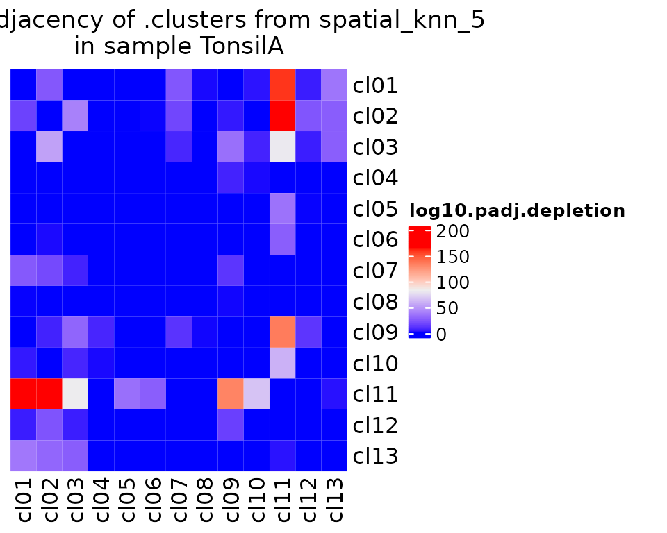
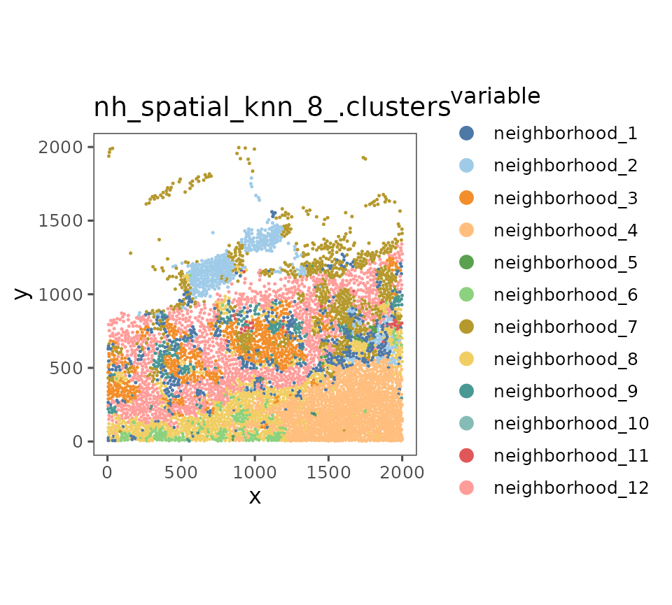
Second, neighborhood analysis, which was described in Schurch et al 2020. Essentially, a nearest neighbor network is computed, the identities of each cell’s neighbors are tallied up, and those vectors are then clustered across the whole dataset. The resulting clusters can be called “neighborhoods” because they describe the overall identity of “windows” of cells.
sm_tonsil <- sm_tonsil %>%
  spatialNearestNeighbors(k = 8) %>%
  cellNeighborhoods(nn = "spatial_knn_8", feature = ".clusters")

sm_tonsil <- neighborhoodClusters(sm_tonsil, nn = "spatial_knn_8", feature = ".clusters")
#> Warning: did not converge in 10 iterations

#> Warning: did not converge in 10 iterations
print(head(cellMetadata(sm_tonsil)))
#>                cell_id        cell.id anno316_some_categories anno916_Leiden_v1
#> TonsilA.125182  125182 TonsilA.125182                     yay         Cluster 2
#> TonsilA.125238  125238 TonsilA.125238                     nay         Cluster 2
#> TonsilA.125254  125254 TonsilA.125254                     yay         Cluster 1
#> TonsilA.125325  125325 TonsilA.125325                     yay         Cluster 1
#> TonsilA.125326  125326 TonsilA.125326                     nay         Cluster 6
#> TonsilA.125608  125608 TonsilA.125608                     nay         Cluster 1
#>                anno248_test_subset_annotation_324
#> TonsilA.125182                                  p
#> TonsilA.125238                                  u
#> TonsilA.125254                                  t
#> TonsilA.125325                                  t
#> TonsilA.125326                                  b
#> TonsilA.125608                                  y
#>                anno1189_uqc_test10_letters_qc_assoc anno1149_uqc_test10_letters
#> TonsilA.125182                                    b                           b
#> TonsilA.125238                                    b                           b
#> TonsilA.125254                                    b                           b
#> TonsilA.125325                                    c                           c
#> TonsilA.125326                                    c                           c
#> TonsilA.125608                                    b                           b
#>                anno1133_uqc_test03_letters anno247_test_letters_324
#> TonsilA.125182                           l                        p
#> TonsilA.125238                           k                        u
#> TonsilA.125254                           z                        t
#> TonsilA.125325                           f                        t
#> TonsilA.125326                           f                        b
#> TonsilA.125608                           m                        y
#>                anno1190_uqc_test10_letters_qc_assoc_postfilt
#> TonsilA.125182                                          <NA>
#> TonsilA.125238                                          <NA>
#> TonsilA.125254                                             b
#> TonsilA.125325                                          <NA>
#> TonsilA.125326                                          <NA>
#> TonsilA.125608                                          <NA>
#>                anno253_Hierarchy.1 anno1797_uqc_test10_letters_221213
#> TonsilA.125182              not Th                                  c
#> TonsilA.125238              not Th                                  b
#> TonsilA.125254    Epithelial Cells                                  b
#> TonsilA.125325    Epithelial Cells                                  b
#> TonsilA.125326   Endothelial Cells                                  b
#> TonsilA.125608    Epithelial Cells                                  b
#>                anno254_Neighborhood.clustering.based.on.annotation.set.253
#> TonsilA.125182                                              neighborhood_2
#> TonsilA.125238                                              neighborhood_2
#> TonsilA.125254                                              neighborhood_0
#> TonsilA.125325                                              neighborhood_0
#> TonsilA.125326                                              neighborhood_2
#> TonsilA.125608                                              neighborhood_0
#>                anno1145_uqc_test08_letters anno1143_uqc_test08_letters  Region
#> TonsilA.125182                           l                           l TonsilA
#> TonsilA.125238                           k                           k TonsilA
#> TonsilA.125254                           z                           z TonsilA
#> TonsilA.125325                           f                           f TonsilA
#> TonsilA.125326                           f                           f TonsilA
#> TonsilA.125608                           m                           m TonsilA
#>                    color width n_channels height
#> TonsilA.125182 grayscale  9408          4   9072
#> TonsilA.125238 grayscale  9408          4   9072
#> TonsilA.125254 grayscale  9408          4   9072
#> TonsilA.125325 grayscale  9408          4   9072
#> TonsilA.125326 grayscale  9408          4   9072
#> TonsilA.125608 grayscale  9408          4   9072
#>                          projection_visualizer_uuid sample_label n_levels
#> TonsilA.125182 96e6af5a-f612-4f97-a294-c580dcd41915  EnableShare        5
#> TonsilA.125238 96e6af5a-f612-4f97-a294-c580dcd41915  EnableShare        5
#> TonsilA.125254 96e6af5a-f612-4f97-a294-c580dcd41915  EnableShare        5
#> TonsilA.125325 96e6af5a-f612-4f97-a294-c580dcd41915  EnableShare        5
#> TonsilA.125326 96e6af5a-f612-4f97-a294-c580dcd41915  EnableShare        5
#> TonsilA.125608 96e6af5a-f612-4f97-a294-c580dcd41915  EnableShare        5
#>                assay_id n_cycles           base_image_visualizer_uuid
#> TonsilA.125182        1        8 728d42b7-77ea-4319-a48a-7f7340bf182d
#> TonsilA.125238        1        8 728d42b7-77ea-4319-a48a-7f7340bf182d
#> TonsilA.125254        1        8 728d42b7-77ea-4319-a48a-7f7340bf182d
#> TonsilA.125325        1        8 728d42b7-77ea-4319-a48a-7f7340bf182d
#> TonsilA.125326        1        8 728d42b7-77ea-4319-a48a-7f7340bf182d
#> TonsilA.125608        1        8 728d42b7-77ea-4319-a48a-7f7340bf182d
#>                experiment_label         segmentation_visualizer_uuid axes
#> TonsilA.125182      enableshare 9d6258e3-1532-40fb-9503-0831f8661358 TCYX
#> TonsilA.125238      enableshare 9d6258e3-1532-40fb-9503-0831f8661358 TCYX
#> TonsilA.125254      enableshare 9d6258e3-1532-40fb-9503-0831f8661358 TCYX
#> TonsilA.125325      enableshare 9d6258e3-1532-40fb-9503-0831f8661358 TCYX
#> TonsilA.125326      enableshare 9d6258e3-1532-40fb-9503-0831f8661358 TCYX
#> TonsilA.125608      enableshare 9d6258e3-1532-40fb-9503-0831f8661358 TCYX
#>                                           assay_metadata assay_description
#> TonsilA.125182 {"image_mpp": 0.377, "num_amp_cycles": 0}
#> TonsilA.125238 {"image_mpp": 0.377, "num_amp_cycles": 0}
#> TonsilA.125254 {"image_mpp": 0.377, "num_amp_cycles": 0}
#> TonsilA.125325 {"image_mpp": 0.377, "num_amp_cycles": 0}
#> TonsilA.125326 {"image_mpp": 0.377, "num_amp_cycles": 0}
#> TonsilA.125608 {"image_mpp": 0.377, "num_amp_cycles": 0}
#>                experiment_id visual_quality assay_name region_display_label
#> TonsilA.125182           164           true      CODEX          EnableShare
#> TonsilA.125238           164           true      CODEX          EnableShare
#> TonsilA.125254           164           true      CODEX          EnableShare
#> TonsilA.125325           164           true      CODEX          EnableShare
#> TonsilA.125326           164           true      CODEX          EnableShare
#> TonsilA.125608           164           true      CODEX          EnableShare
#>                biomarker_expression_version segmentation_version    study_name
#> TonsilA.125182                            1                    1 Enable Tonsil
#> TonsilA.125238                            1                    1 Enable Tonsil
#> TonsilA.125254                            1                    1 Enable Tonsil
#> TonsilA.125325                            1                    1 Enable Tonsil
#> TonsilA.125326                            1                    1 Enable Tonsil
#> TonsilA.125608                            1                    1 Enable Tonsil
#>                coverslip_id cellqc_signal.sum cellqc_signal.mean
#> TonsilA.125182          164          2150.384           134.3990
#> TonsilA.125238          164          1643.021           102.6888
#> TonsilA.125254          164          5008.782           313.0489
#> TonsilA.125325          164          4780.682           298.7926
#> TonsilA.125326          164          2061.935           128.8709
#> TonsilA.125608          164          2562.896           160.1810
#>                cellqc_signal.min cellqc_signal.max cellqc_signal.median
#> TonsilA.125182            25.351           616.531              71.2760
#> TonsilA.125238            22.278           264.544              94.6020
#> TonsilA.125254            43.392          1176.123             186.8460
#> TonsilA.125325            43.724          1091.923             216.6215
#> TonsilA.125326            26.698           333.908              84.0285
#> TonsilA.125608            27.512           415.596             135.3460
#>                cellqc_signal.sd cellqc_signal.vars cellqc_DNA cellqc_cell.size
#> TonsilA.125182        156.32565          24437.708   2711.271              484
#> TonsilA.125238         75.59541           5714.666   1606.299              763
#> TonsilA.125254        358.27940         128364.126   1644.679              357
#> TonsilA.125325        304.16653          92517.280   1650.913              417
#> TonsilA.125326         99.92029           9984.064   2454.006              520
#> TonsilA.125608        116.45369          13561.462   2145.376              651
#>                cellqc_signal.cv .pass_qc            .qc_result .clusters
#> TonsilA.125182        1.1631459    FALSE            signal.sum      cl01
#> TonsilA.125238        0.7361601    FALSE signal.sum, signal.cv      cl01
#> TonsilA.125254        1.1444839     TRUE                  pass      cl02
#> TonsilA.125325        1.0179854     TRUE                  pass      cl03
#> TonsilA.125326        0.7753516    FALSE            signal.sum      cl04
#> TonsilA.125608        0.7270131    FALSE             signal.cv      cl01
#>                Cell.type nh_spatial_knn_8_.clusters
#> TonsilA.125182    B Cell            neighborhood_10
#> TonsilA.125238    B Cell            neighborhood_10
#> TonsilA.125254    T Cell            neighborhood_10
#> TonsilA.125325      <NA>            neighborhood_10
#> TonsilA.125326      <NA>            neighborhood_10
#> TonsilA.125608    B Cell            neighborhood_10

plotRepresentation(sm_tonsil[[1]], "spatial", "nh_spatial_knn_8_.clusters")