Package emobject
![]()
emObject Guide
![]()
What is emObject?
emObject is an abstraction for multimodal spatial omics data in Python. It’s inspired by other data abstractions and data science libraries like Seurat, but purpose-built for multiplexed imaging, spatial transcriptomics, and similar assays. emObject unlocks a seamless data science workflow between the core data types in a spatial dataset: matrix-format data, images, and masks - via shared indexing and dedicated attributes to hold measurements, featurizations, and annotations on data across spatial scales.
As emObject evolves, we envision this data abstraction providing an expected and efficient format for science and engineering code and as a step towards closing the loop between code and no-code analysis on the Enable platform.
For more info about the design and motivation for emObject, see the manuscript emObject: domain specific data abstraction for spatial omics.
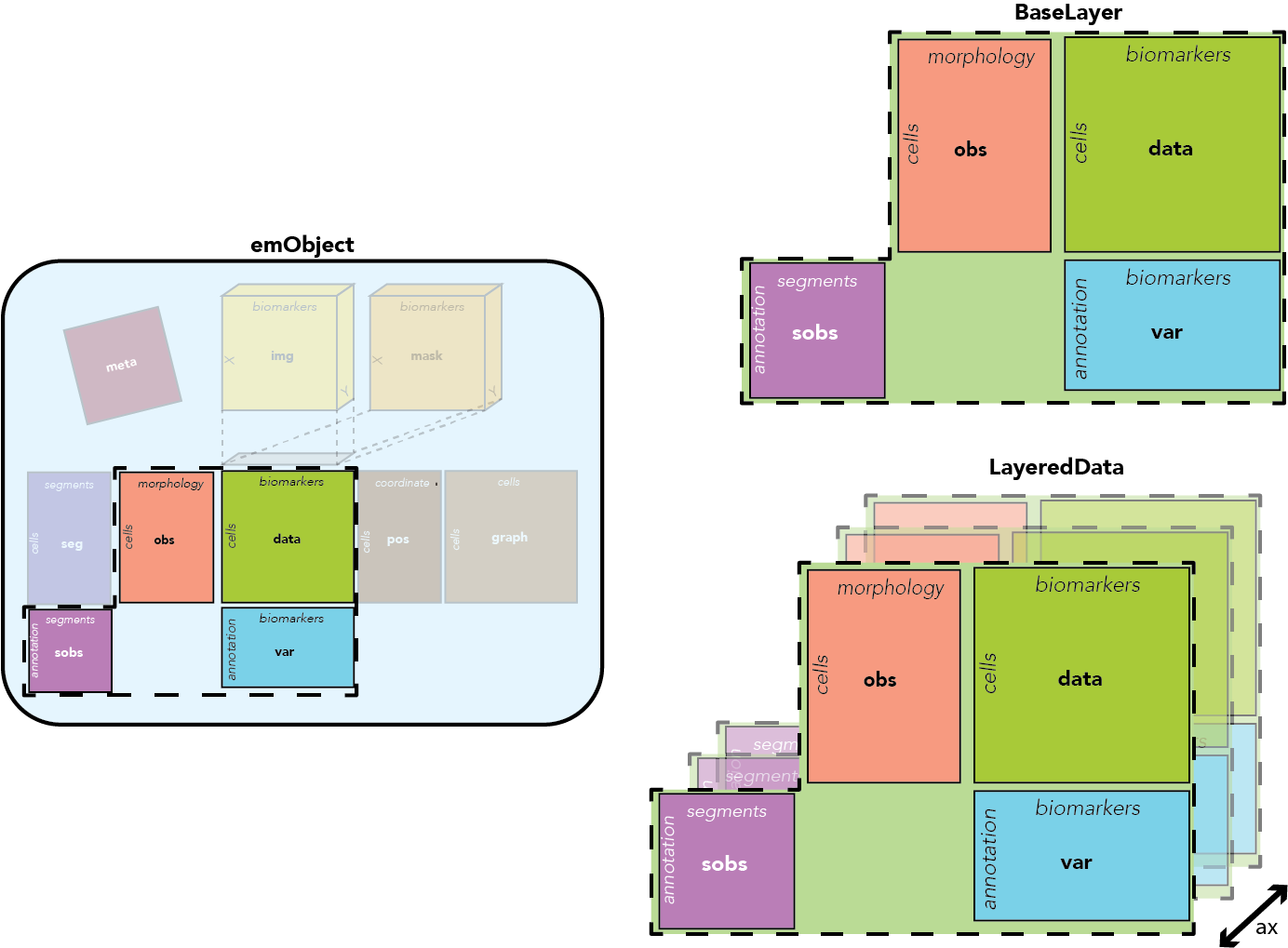
What’s in an emObject?
emObject has dedicated attributes for all the common attributes we encounter in analyzing spatial data. A single emObject represents data at the acquisition level - future functionality is planned to represent experiments.
Data attributes are aligned along several axes:
- The observation axis - typically cells or visium spots
- The variable axis - typically genes or biomarkers
- The segment axis - unique, contiguous regions of ROI masks
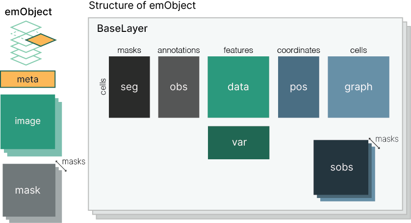
Layers
Layers are an additional axis within emObjects that stack the core data attributes - data, var, obs, sobs. This allows us to hold multiple versions - or multiple data modalities - within a single object. For example, we could have a raw and normalized data layer, or a layer for CODEX and a layer for H+E data. Annotations are kept within a layer since computations derived from the images may be affected by the numeric values in data.
What gets stored where?
- Biomarker expression -> data
- Notes about biomarkers -> var
- Featurization -> obs
- Spatial info -> pos
- Assignment of cells to segments -> seg
- Annotations on segment level -> sobs
- Unstructured info, whole image annotations -> meta
Getting started
Requirements
emObject requires Python 3.8 or higher and is tested on MacOS 13.2 (Ventura) and Ubuntu 18.04 and 22.04.
Installation
To install emObject, clone this repo:
git clone https://gitlab.com/enable-medicine-public/emobject.git
and install:
sudo python setup.py install
If you use pipenv as a package manager, you can install via:
pipenv install '-e .' --dev
from within the emobject.emobject repository.
You can also install directly via PyPI:
pip install emobject
or, if you use pipenv (recommended):
pipenv install emobject
emObject API
Overview
emObject strives to maintain consistency with existing tools in the Python data science ecosystem, like Pandas and NumPy. Wherever possible, the API is shared - under the hood, many attributes of emObject rely on existing tools. When we need to introduce something new, an effort is made to design an API that feels familiar to users comfortable with the Python data science ecosystem.
Tutorial
A full demo is available on Gitlab.
import emobject.emobject as emo
import emobject.emimage as emi
from emobject import core
import pandas as pd
import numpy as np
import matplotlib.pyplot as plt

import os
🏗️ Building an EMObject
There are several ways to construct an EMObject. We provide an API for building an EMObject directly from the Enable Database (currently for Enable internal users only) and reading EMObjects from an on-disk store.
It's also possible to directly create an EMObject from existing data you might have, but this currently requires a good understanding of EMObject's inner workings and can lead to unexpected behavior if done incorrectly. We're working to streamline this, so in the meantime it is highly recommended to use one of the above options.
💽 Loading an EMObject from Disk
We
can load an existing EMObject from its on-disk Zarr representation.
E = core.load('./test/Charville_c001_v001_r001_reg001.zarr/')
🔎 Access object attributes
Most attributes are represented as Pandas DataFrames, and can be interacted with using standard Pandas API. For example, we can grab the first 10 biomarker expression entries:
E.data.head(10)
| ACE2 | C1QC | C3a | C3aR | C3d | C4d | C5aR | C9 | CD107a | CD11b | ... | Nestin | PD1 | Perlecan | RORgammaT | SC5b9 | SPP1 | TFAM | VWF | aSMA | bCatenin1 | |
|---|---|---|---|---|---|---|---|---|---|---|---|---|---|---|---|---|---|---|---|---|---|
| 0 | 49.587002 | 54.153999 | 25.731001 | 32.875000 | 189.759995 | 123.827003 | 81.125000 | 2032.095947 | 43.009998 | 33.596001 | ... | 53.019001 | 27.941999 | 120.721001 | 1796.962036 | 58.250000 | 153.837006 | 89.875000 | 64.231003 | 1747.692017 | 75.077003 |
| 1 | 44.856998 | 44.034000 | 27.017000 | 32.882000 | 158.738998 | 54.175999 | 102.570999 | 228.285995 | 84.403000 | 37.251999 | ... | 147.798004 | 24.118000 | 55.630001 | 1120.470947 | 60.546001 | 157.419998 | 180.007996 | 53.890999 | 51.437000 | 101.235001 |
| 2 | 40.327999 | 310.492004 | 32.770000 | 40.984001 | 138.893005 | 106.171997 | 85.630997 | 372.106995 | 297.024994 | 41.344002 | ... | 132.712997 | 27.007999 | 31.556999 | 1685.836060 | 56.492001 | 249.188995 | 216.753998 | 75.320000 | 74.762001 | 111.671997 |
| 3 | 20.856001 | 166.123993 | 25.691000 | 25.660000 | 160.227005 | 107.856003 | 68.732002 | 243.763000 | 365.947998 | 31.732000 | ... | 81.556999 | 36.041000 | 27.237000 | 1615.979004 | 49.845001 | 178.619003 | 301.082001 | 49.289001 | 53.535999 | 177.505005 |
| 4 | 43.766998 | 60.401001 | 33.076000 | 31.785000 | 141.186005 | 65.016998 | 90.372002 | 193.070007 | 127.348999 | 34.570000 | ... | 38.145000 | 27.563999 | 104.070000 | 953.093018 | 69.453003 | 174.285004 | 143.947998 | 45.942001 | 2774.000000 | 63.772999 |
| 5 | 76.591003 | 141.460007 | 33.549000 | 33.390999 | 101.567001 | 97.920998 | 110.177002 | 824.818970 | 73.577003 | 47.869999 | ... | 38.980999 | 17.847000 | 31.004999 | 1290.237061 | 21.698000 | 122.609001 | 312.526001 | 40.186001 | 69.702003 | 186.623001 |
| 6 | 48.544998 | 76.192001 | 51.222000 | 30.365000 | 106.832001 | 81.598999 | 55.222000 | 725.395020 | 135.753998 | 27.347000 | ... | 169.240005 | 28.671000 | 139.759995 | 1098.677002 | 43.849998 | 138.042007 | 136.634995 | 44.922001 | 78.089996 | 98.371002 |
| 7 | 36.069000 | 129.701996 | 33.122002 | 33.744999 | 92.988998 | 56.734001 | 73.181000 | 275.505005 | 97.441002 | 33.605999 | ... | 51.590000 | 24.979000 | 51.355999 | 925.956970 | 65.185997 | 101.169998 | 145.207001 | 34.431000 | 57.931000 | 119.323997 |
| 8 | 48.678001 | 201.602005 | 30.000000 | 51.279999 | 71.415001 | 46.279999 | 31.424000 | 350.524994 | 230.643997 | 33.144001 | ... | 33.202999 | 29.322001 | 57.126999 | 990.280029 | 59.431999 | 238.914993 | 554.711975 | 149.686005 | 249.085007 | 510.135986 |
| 9 | 33.963001 | 315.472992 | 29.316000 | 29.952000 | 126.676003 | 86.385002 | 76.329002 | 313.748993 | 143.979004 | 39.532001 | ... | 131.382004 | 26.877001 | 65.388000 | 1366.035034 | 70.013000 | 362.824005 | 236.968002 | 82.174004 | 54.801998 | 169.591003 |
10 rows × 42 columns
Data and attributes are indexed by the observeration axis (cells) and the variable axis (biomarkers/genes). In some cases, no axis is provided, in which case an integer axis is generated. To inspect the axes:
E.obs_ax
RangeIndex(start=0, stop=10145, step=1)
EMObject attributes are built on top of familiar libraries from the Python data science ecosystem, like NumPy and Pandas. This gives EMObject data attrbutes a familiar API. For example, we can slice through individual attributes using Pandas .loc:
E.data.loc[:,'CD45']
0        107.672997
1        100.445000
2        156.197006
3        150.371002
4        100.744003
            ...
10140    166.009995
10141    174.339005
10142    106.834999
10143    302.000000
10144     62.540001
Name: CD45, Length: 10145, dtype: float64
Annotations about observations are stored in .obs.
E.obs.head(10)
| VALUE | ANNOTATION_LABEL | |
|---|---|---|
| 0 | 1 | cl04 |
| 1 | 16 | cl08 |
| 2 | 6 | cl12 |
| 3 | 6 | cl12 |
| 4 | 1 | cl04 |
| 5 | 5 | cl06 |
| 6 | 3 | cl07 |
| 7 | 6 | cl12 |
| 8 | 4 | cl10 |
| 9 | 6 | cl12 |
✏️ Annotating EMObject Attributes
In our object, we didn't provide any annotations to variables, but they can be stored in .var. No attributes are created until called, so this adds no overhead until used:
E.var.head(10)
| ACE2 |
|---|
| C1QC |
| C3a |
| C3aR |
| C3d |
| C4d |
| C5aR |
| C9 |
| CD107a |
| CD11b |
But, we could add some annotation to the biomarkers
passed_qc = np.random.randint(0, 2, size=E.var_ax.shape[0]) # some dummy values
passed_qc = passed_qc.astype(bool)
E.add_anno(
    attr='var',
    value=passed_qc,
    name="PassedQC")
E.var.head(5)
| PassedQC | |
|---|---|
| ACE2 | True |
| C1QC | True |
| C3a | False |
| C3aR | True |
| C3d | True |
You can do this on observations too.
random_int = np.random.randint(0, 10, size=E.n_obs)

E.add_anno(
    attr='obs',
    value=random_int,
    name='RandomIntAnno'
)
E.obs.head(10)
| VALUE | ANNOTATION_LABEL | RandomIntAnno | |
|---|---|---|---|
| 0 | 1 | cl04 | 7 |
| 1 | 16 | cl08 | 2 |
| 2 | 6 | cl12 | 4 |
| 3 | 6 | cl12 | 6 |
| 4 | 1 | cl04 | 3 |
| 5 | 5 | cl06 | 2 |
| 6 | 3 | cl07 | 8 |
| 7 | 6 | cl12 | 8 |
| 8 | 4 | cl10 | 3 |
| 9 | 6 | cl12 | 5 |
You could also add 2-D arrays of annotations:
multiple_annos = np.random.randint(0,100, (E.n_obs, 2))
multiple_annos
array([[92,  5],
       [21, 77],
       [94, 18],
       ...,
       [14,  4],
       [46, 64],
       [27, 51]])
multiple_annos = np.random.randint(0,100, (E.n_obs, 2))

E.add_anno(
    attr='obs',
    value=multiple_annos,
    name=['test1', 'test2']
)

E.obs.head(5)
| VALUE | ANNOTATION_LABEL | RandomIntAnno | test1 | test2 | |
|---|---|---|---|---|---|
| 0 | 1 | cl04 | 7 | 19 | 50 |
| 1 | 16 | cl08 | 2 | 14 | 13 |
| 2 | 6 | cl12 | 4 | 23 | 99 |
| 3 | 6 | cl12 | 6 | 36 | 64 |
| 4 | 1 | cl04 | 3 | 40 | 88 |
E.obs
| VALUE | ANNOTATION_LABEL | RandomIntAnno | test1 | test2 | |
|---|---|---|---|---|---|
| 0 | 1 | cl04 | 7 | 19 | 50 |
| 1 | 16 | cl08 | 2 | 14 | 13 |
| 2 | 6 | cl12 | 4 | 23 | 99 |
| 3 | 6 | cl12 | 6 | 36 | 64 |
| 4 | 1 | cl04 | 3 | 40 | 88 |
| ... | ... | ... | ... | ... | ... |
| 10140 | 4 | cl10 | 9 | 19 | 35 |
| 10141 | 4 | cl10 | 9 | 19 | 93 |
| 10142 | 12 | cl15 | 3 | 7 | 41 |
| 10143 | 0 | cl01 | 8 | 81 | 80 |
| 10144 | 13 | cl16 | 7 | 5 | 36 |
10145 rows × 5 columns
🤿 Working with ROI and segmentation masks
Masks are stored in .mask, but are represented as a unique EMMask object.
We see that this object has 3 masks associated with it.
E.mask.n_masks
3
If you're loading an EMObject from a previous store or the Enable database, you'll see whatever names were stored last. The segmentation mask you've requested will always be named segmentation_mask.
We're building from scratch, so EMObject has provided dummy mask names, which we can update.
E.mask.mask_names
array(['mask_0', 'mask_1', 'mask_2'], dtype='<U6')
E.mask.mask_names = np.array(['gloms', 'bloodvessels', 'artifacts'])
Masks can be selected by name with an interface similar to Pandas:
E.mask.mloc('gloms')
array([], shape=(0, 4032, 4032), dtype=int64)
To plot a mask:
E.mask.plot('gloms')

🧩 Segments
Within masks, each contiguous region is defined as a segment. For example, in the mask shown above, there are 3 segments.
To enable segment-wise annotations and analysis, we generate a mapping of observatoins to segments, in .seg, which is a n_obs x n_mask array. Non-zero elements of .seg are unique identifiers of segment. The col index of .seg matches the .mask index.
A summary of mask segments is provided in the n_seg attribute:
E.n_seg
{'gloms': 3, 'bloodvessels': 4, 'artifacts': 1}
E.seg
array([[   0, 9479,    0],
       [   0,    0,    0],
       [   0,    0,    0],
       ...,
       [   0,    0,    0],
       [   0,    0,    0],
       [   0,    0,    0]], dtype=uint16)
As with other types of data, EMObject supports annotations on segments via the add_anno and del_anno functions previously described.
Because sobs stores an annotation array per mask, we must specify the mask. A current quirk is that calls to sobs arrays in the object (e.g. to read them) must be done by index. API improvements incoming here.
seg_anno = np.random.randint(0, 100, 4)

E.add_anno(
    attr='sobs',
    value=seg_anno,
    name='TestSegAnno',
    mask='gloms'
)

E.sobs[0]
| TestSegAnno | |
|---|---|
| 0 | 35 |
| 9637 | 73 |
| 9638 | 29 |
| 9639 | 36 |
Now delete it:
E.del_anno(
    attr='sobs',
    name='TestSegAnno',
    mask='gloms'
)
🥞 Layering
EMObject supports layers, which are intended to hold transformations on the core data within one object. For example, the same region could have the original raw data matrix, plus a normalized transformation of that data. It's also possible that derived measurments on observations or variables could be affected by the original data.
BaseLayer contains all of the core tabular data attributes of EMObject: data, obs, var. EMObject wraps multiple BaseLayers into LayeredData, which allows for indexing along a layer axis. You don't really need to know how this works because you can interact as if it's all one object. If you only dream of one layer, all of the above still works (we've been using LayeredData the whole time).
To illustrate, we'll define a trivial transformation on our data:
normed_data = (E.data-E.data.mean())/E.data.std()
Now, we can add this data to a new BaseLayer called 'z-normed'.
from emobject.emlayer import BaseLayer

normed_layer = BaseLayer(data=normed_data,
                         name = 'z-normed')
We can add this BaseLayer to our EMObject.
E.add(normed_layer)
To see the layers associated with your EMObject:
E.layers
['raw', 'z-normed']
By default, our original data is stored in the raw layer. We can see that we've now added a layer z-normed.
We can specify which layer we want to work inside of:
E.set_layer('z-normed')
Let's take a look at the data in the layer. It should match our transformed data above.
E.data
| ACE2 | C1QC | C3a | C3aR | C3d | C4d | C5aR | C9 | CD107a | CD11b | ... | Nestin | PD1 | Perlecan | RORgammaT | SC5b9 | SPP1 | TFAM | VWF | aSMA | bCatenin1 | |
|---|---|---|---|---|---|---|---|---|---|---|---|---|---|---|---|---|---|---|---|---|---|
| 0 | 0.861139 | -0.553432 | -1.128674 | 0.667163 | 1.865417 | 2.651764 | -0.004316 | 0.653558 | -1.140414 | -0.234559 | ... | 0.045634 | 0.938042 | 1.439976 | 1.874962 | 0.025475 | -0.302155 | -0.743126 | 0.205744 | 7.907488 | -0.786248 |
| 1 | 0.120701 | -0.603356 | -1.040028 | 0.668495 | 0.955026 | -0.729141 | 1.768532 | -0.400150 | -0.726064 | -0.142371 | ... | 2.599334 | -0.094610 | -0.285497 | 0.393158 | 0.227152 | -0.269929 | -0.119544 | -0.280852 | -0.644272 | -0.441339 |
| 2 | -0.588271 | 0.711128 | -0.643469 | 2.209511 | 0.372595 | 1.794778 | 0.368175 | -0.316135 | 1.402313 | -0.039190 | ... | 2.192888 | 0.685820 | -0.923639 | 1.631549 | -0.128945 | 0.555452 | 0.134682 | 0.727588 | -0.526678 | -0.303720 |
| 3 | -3.636431 | -0.001065 | -1.131431 | -0.705144 | 0.998696 | 1.876521 | -1.028792 | -0.391109 | 2.092243 | -0.281560 | ... | 0.814554 | 3.125138 | -1.038156 | 1.478532 | -0.712807 | -0.079263 | 0.718102 | -0.497420 | -0.633690 | 0.564328 |
| 4 | -0.049928 | -0.522615 | -0.622376 | 0.459843 | 0.439889 | -0.202912 | 0.760093 | -0.420721 | -0.296168 | -0.209999 | ... | -0.355127 | 0.835965 | 0.998581 | 0.026529 | 1.009529 | -0.118243 | -0.369024 | -0.654928 | 13.081675 | -0.935298 |
| ... | ... | ... | ... | ... | ... | ... | ... | ... | ... | ... | ... | ... | ... | ... | ... | ... | ... | ... | ... | ... | ... |
| 10140 | 0.794765 | -0.156100 | -1.010940 | 0.158564 | -1.336108 | -0.460129 | 0.213425 | -0.331019 | 0.727229 | -0.066397 | ... | -0.697663 | -1.828570 | -0.196985 | -0.710627 | -0.527116 | 0.555893 | 1.733469 | 0.917237 | -0.473056 | 3.632792 |
| 10141 | -0.944245 | 0.100189 | -0.841783 | 1.503291 | 0.265682 | 2.088207 | -0.819400 | -0.310262 | 0.058562 | -0.250722 | ... | -0.809614 | -1.224209 | -0.552598 | 0.836100 | -0.900781 | 0.550002 | 2.029655 | 0.300475 | -0.675928 | 0.800746 |
| 10142 | -0.723053 | 0.448905 | 1.459957 | -0.320936 | -0.648289 | -0.274315 | -0.912647 | 0.237139 | -1.004225 | -0.105759 | ... | -0.373206 | 0.106573 | -0.270679 | -0.344543 | -1.635813 | -0.577186 | -0.322158 | 0.163014 | -0.205314 | -0.679154 |
| 10143 | -3.000876 | 6.696201 | 0.749141 | 1.710801 | -2.523276 | -2.463839 | -1.745421 | -0.189334 | -0.870920 | -0.169478 | ... | -0.257725 | 0.167873 | -0.736223 | 0.146715 | -3.137586 | 0.627325 | 1.880645 | -0.150450 | 0.256336 | -0.974552 |
| 10144 | 0.563085 | -0.446397 | 0.908165 | 0.864593 | -1.196649 | -1.614717 | -2.613742 | 7.859175 | -0.999621 | -0.254756 | ... | -0.326055 | 1.168391 | -0.093919 | -0.809684 | -1.061438 | -0.847937 | -0.778016 | -1.080723 | 0.664329 | -0.582675 |
10145 rows × 42 columns
We haven't defined any variable annotations on this layer, so we shouldn't see any if we check:
E.var.head(5)
| ACE2 |
|---|
| C1QC |
| C3a |
| C3aR |
| C3d |
We revert back to the original annotations provided at object construction time, here we should just see ANNOTATION_LABEL, but nothing else that we've added in the previous steps.
E.obs
| VALUE | ANNOTATION_LABEL | |
|---|---|---|
| 0 | 1 | cl04 |
| 1 | 16 | cl08 |
| 2 | 6 | cl12 |
| 3 | 6 | cl12 |
| 4 | 1 | cl04 |
| ... | ... | ... |
| 10140 | 4 | cl10 |
| 10141 | 4 | cl10 |
| 10142 | 12 | cl15 |
| 10143 | 0 | cl01 |
| 10144 | 13 | cl16 |
10145 rows × 2 columns
We can still add annotations as described above:
random_int = np.random.randint(30, 70, size=E.n_obs)

E.add_anno(
    attr='obs',
    value=random_int,
    name='RandomIntAnno - Layer'
)
E.obs.head(10)
| VALUE | ANNOTATION_LABEL | RandomIntAnno - Layer | |
|---|---|---|---|
| 0 | 1 | cl04 | 59 |
| 1 | 16 | cl08 | 67 |
| 2 | 6 | cl12 | 49 |
| 3 | 6 | cl12 | 68 |
| 4 | 1 | cl04 | 44 |
| 5 | 5 | cl06 | 43 |
| 6 | 3 | cl07 | 68 |
| 7 | 6 | cl12 | 30 |
| 8 | 4 | cl10 | 69 |
| 9 | 6 | cl12 | 43 |
You can change layers using .set_layer. Passing no args will return you to the starting layer.
E.set_layer()
…and we're back to our raw data annotations
E.obs.head(10)
| VALUE | ANNOTATION_LABEL | RandomIntAnno | test1 | test2 | |
|---|---|---|---|---|---|
| 0 | 1 | cl04 | 7 | 19 | 50 |
| 1 | 16 | cl08 | 2 | 14 | 13 |
| 2 | 6 | cl12 | 4 | 23 | 99 |
| 3 | 6 | cl12 | 6 | 36 | 64 |
| 4 | 1 | cl04 | 3 | 40 | 88 |
| 5 | 5 | cl06 | 2 | 33 | 59 |
| 6 | 3 | cl07 | 8 | 66 | 89 |
| 7 | 6 | cl12 | 8 | 90 | 69 |
| 8 | 4 | cl10 | 3 | 76 | 40 |
| 9 | 6 | cl12 | 5 | 28 | 32 |
🍕 Slicing
EMObject also supports slicing, using a Pandas-like notation. Slicing an object returns an in-memory view of the current layer, with data attributes subsetted to your specifications.
obs_subset = np.arange(0, E.n_obs, 32) # get every 32nd cell in the object
var_subset = np.array(['DAPI', 'CD45', 'aSMA']) # our favorite markers

E_subset = E.loc(obs_subset=obs_subset,
                 var_subset=var_subset)
We should see that our object attributes have been subsetted:
E_subset.data
| DAPI | CD45 | aSMA | |
|---|---|---|---|
| 0 | 1395.125000 | 107.672997 | 1747.692017 |
| 32 | 533.392029 | 82.212997 | 384.036011 |
| 64 | 441.308990 | 132.386002 | 84.008003 |
| 96 | 435.066986 | 211.649994 | 100.272003 |
| 128 | 1069.602051 | 97.053001 | 200.548996 |
| ... | ... | ... | ... |
| 10016 | 484.878998 | 112.075996 | 324.112000 |
| 10048 | 380.605011 | 176.182999 | 50.473000 |
| 10080 | 446.473999 | 297.463013 | 49.445999 |
| 10112 | 697.681030 | 495.598999 | 146.701996 |
| 10144 | 453.708008 | 62.540001 | 311.000000 |
318 rows × 3 columns
E_subset.obs
| VALUE | ANNOTATION_LABEL | RandomIntAnno | test1 | test2 | |
|---|---|---|---|---|---|
| 0 | 1 | cl04 | 7 | 19 | 50 |
| 32 | 1 | cl04 | 1 | 30 | 87 |
| 64 | 4 | cl10 | 0 | 78 | 20 |
| 96 | 6 | cl12 | 9 | 18 | 57 |
| 128 | 5 | cl06 | 1 | 9 | 53 |
| ... | ... | ... | ... | ... | ... |
| 10016 | 13 | cl16 | 9 | 86 | 53 |
| 10048 | 0 | cl01 | 9 | 22 | 73 |
| 10080 | 6 | cl12 | 2 | 18 | 42 |
| 10112 | 8 | cl09 | 6 | 69 | 42 |
| 10144 | 13 | cl16 | 7 | 5 | 36 |
318 rows × 5 columns
E_subset.pos
| X | Y | |
|---|---|---|
| 0 | 1249 | 3 |
| 32 | 1356 | 19 |
| 64 | 2457 | 46 |
| 96 | 2528 | 66 |
| 128 | 1236 | 85 |
| ... | ... | ... |
| 10016 | 1465 | 3920 |
| 10048 | 1661 | 3942 |
| 10080 | 1891 | 3968 |
| 10112 | 1569 | 3998 |
| 10144 | 1241 | 4027 |
318 rows × 2 columns
We can also slice through on the basis of cells or masks:
glom_data = E.loc(mask='gloms')
glom_data.data.head()
| ACE2 | C1QC | C3a | C3aR | C3d | C4d | C5aR | C9 | CD107a | CD11b | ... | Nestin | PD1 | Perlecan | RORgammaT | SC5b9 | SPP1 | TFAM | VWF | aSMA | bCatenin1 | |
|---|---|---|---|---|---|---|---|---|---|---|---|---|---|---|---|---|---|---|---|---|---|
| 4341 | 39.344002 | 45.964001 | 33.146999 | 26.254000 | 112.846001 | 58.304001 | 79.098000 | 735.867981 | 133.570999 | 38.376999 | ... | 41.230000 | 19.122999 | 73.546997 | 444.032990 | 55.625000 | 109.775002 | 90.346001 | 38.042000 | 166.102997 | 69.765999 |
| 4342 | 43.320000 | 62.255001 | 37.923000 | 31.138000 | 168.177002 | 79.013000 | 82.688004 | 330.763000 | 80.392998 | 40.320000 | ... | 69.781998 | 24.738001 | 72.544998 | 882.987976 | 62.062000 | 143.921997 | 101.931999 | 42.033001 | 89.245003 | 77.458000 |
| 4345 | 49.942001 | 56.445000 | 36.929001 | 29.909000 | 103.776001 | 61.101002 | 71.662003 | 463.364014 | 143.815002 | 36.234001 | ... | 93.794998 | 24.827999 | 82.416000 | 768.776001 | 42.035999 | 115.320999 | 83.938004 | 51.294998 | 77.350998 | 101.653000 |
| 4359 | 41.818001 | 46.442001 | 39.831001 | 33.262001 | 89.917000 | 57.213001 | 69.768997 | 564.530029 | 92.921997 | 39.608002 | ... | 50.088001 | 25.851999 | 56.330002 | 531.231018 | 53.527000 | 118.481003 | 89.055000 | 31.743000 | 88.074997 | 77.803001 |
| 4384 | 45.422001 | 54.389999 | 33.090000 | 21.351999 | 99.578003 | 41.410000 | 83.872002 | 889.322998 | 132.026001 | 35.235001 | ... | 34.358002 | 24.080999 | 70.692001 | 367.859985 | 52.395000 | 74.615997 | 83.956001 | 41.930000 | 266.415985 | 71.622002 |
5 rows × 42 columns
segment_data = E.loc(seg_subset=9479)
segment_data.obs
| VALUE | ANNOTATION_LABEL | RandomIntAnno | test1 | test2 | |
|---|---|---|---|---|---|
| 0 | 1 | cl04 | 7 | 19 | 50 |
| 39 | 1 | cl04 | 4 | 45 | 80 |
| 47 | 13 | cl16 | 7 | 38 | 16 |
| 61 | 1 | cl04 | 6 | 80 | 74 |
| 84 | 1 | cl04 | 7 | 42 | 52 |
You can also use slicing notation on the EMObject directly to access layers:
E['z-normed'].data.head(10)
| ACE2 | C1QC | C3a | C3aR | C3d | C4d | C5aR | C9 | CD107a | CD11b | ... | Nestin | PD1 | Perlecan | RORgammaT | SC5b9 | SPP1 | TFAM | VWF | aSMA | bCatenin1 | |
|---|---|---|---|---|---|---|---|---|---|---|---|---|---|---|---|---|---|---|---|---|---|
| 0 | 0.861139 | -0.553432 | -1.128674 | 0.667163 | 1.865417 | 2.651764 | -0.004316 | 0.653558 | -1.140414 | -0.234559 | ... | 0.045634 | 0.938042 | 1.439976 | 1.874962 | 0.025475 | -0.302155 | -0.743126 | 0.205744 | 7.907488 | -0.786248 |
| 1 | 0.120701 | -0.603356 | -1.040028 | 0.668495 | 0.955026 | -0.729141 | 1.768532 | -0.400150 | -0.726064 | -0.142371 | ... | 2.599334 | -0.094610 | -0.285497 | 0.393158 | 0.227152 | -0.269929 | -0.119544 | -0.280852 | -0.644272 | -0.441339 |
| 2 | -0.588271 | 0.711128 | -0.643469 | 2.209511 | 0.372595 | 1.794778 | 0.368175 | -0.316135 | 1.402313 | -0.039190 | ... | 2.192888 | 0.685820 | -0.923639 | 1.631549 | -0.128945 | 0.555452 | 0.134682 | 0.727588 | -0.526678 | -0.303720 |
| 3 | -3.636431 | -0.001065 | -1.131431 | -0.705144 | 0.998696 | 1.876521 | -1.028792 | -0.391109 | 2.092243 | -0.281560 | ... | 0.814554 | 3.125138 | -1.038156 | 1.478532 | -0.712807 | -0.079263 | 0.718102 | -0.497420 | -0.633690 | 0.564328 |
| 4 | -0.049928 | -0.522615 | -0.622376 | 0.459843 | 0.439889 | -0.202912 | 0.760093 | -0.420721 | -0.296168 | -0.209999 | ... | -0.355127 | 0.835965 | 0.998581 | 0.026529 | 1.009529 | -0.118243 | -0.369024 | -0.654928 | 13.081675 | -0.935298 |
| 5 | 5.088364 | -0.122737 | -0.589772 | 0.765307 | -0.722832 | 1.394270 | 2.397287 | -0.051681 | -0.834433 | 0.125366 | ... | -0.332602 | -1.788064 | -0.938272 | 0.765018 | -3.185195 | -0.583024 | 0.797277 | -0.925803 | -0.552188 | 0.684555 |
| 6 | 0.698023 | -0.444715 | 0.628443 | 0.189757 | -0.568317 | 0.601989 | -2.145606 | -0.109760 | -0.212033 | -0.392130 | ... | 3.177062 | 1.134905 | 1.944673 | 0.345420 | -1.239398 | -0.444217 | -0.419619 | -0.702929 | -0.509899 | -0.479102 |
| 7 | -1.254978 | -0.180741 | -0.619205 | 0.832639 | -0.974576 | -0.604974 | -0.661013 | -0.372566 | -0.595551 | -0.234307 | ... | 0.007132 | 0.137898 | -0.398795 | -0.032911 | 0.634722 | -0.775849 | -0.360313 | -1.196631 | -0.611532 | -0.202824 |
| 8 | 0.718843 | 0.173954 | -0.834408 | 4.167830 | -1.607720 | -1.112418 | -4.112884 | -0.328743 | 0.737830 | -0.245956 | ... | -0.488283 | 1.310705 | -0.245814 | 0.107984 | 0.129300 | 0.463047 | 2.472831 | 4.227219 | 0.352181 | 4.950272 |
| 9 | -1.584653 | 0.735700 | -0.881556 | 0.111203 | 0.014056 | 0.834305 | -0.400781 | -0.350226 | -0.129699 | -0.084880 | ... | 2.157026 | 0.650444 | -0.026826 | 0.931048 | 1.058718 | 1.577500 | 0.274532 | 1.050134 | -0.627307 | 0.459977 |
10 rows × 42 columns
🔬 Accessing images
EMObject represents images as an in-memory or on-disk Zarr hierarchy using the EMImage class. You can access the image directly, plot channels, and use for downstream analysis.
See what channels are in this image:
E.img.channels
array(['ACE2', 'C1QC', 'C3a', 'C3aR', 'C3d', 'C4d', 'C5aR', 'C9',
       'CD107a', 'CD11b', 'CD11c', 'CD141', 'CD183', 'CD196', 'CD21',
       'CD227', 'CD25', 'CD31', 'CD35', 'CD38', 'CD45', 'CD46', 'CD55',
       'CD68', 'Clusterin', 'CollagenIV', 'DAPI', 'EpCAM', 'FoxP3',
       'GranzymeB', 'ICOS', 'MASP2', 'Nestin', 'PD1', 'Perlecan',
       'RORgammaT', 'SC5b9', 'SPP1', 'TFAM', 'VWF', 'aSMA', 'bCatenin1'],
      dtype=object)
Plot an image channel:
E.img.plot_channel('DAPI')

E.img.img
<zarr.core.Array (42, 4032, 4032) uint16>
💾 Saving EMObjects to disk
EMObjects can be saved to disk as a Zarr store.
core.save(E, out_dir='./savetest')
We can also verify that this object is what we think we saved:
E2 = core.load('./savetest/DemoKidney.zarr/')
E2.summary
EMObject Version 0.4.0
EMObject:
Layers: 2
     Layer 1: raw
     Layer 2: z-normed
obs: 10145
var: 42
masks: 3
Issues and Contributions
emObject is very young 🐣! If you encounter a bug or missing/desired functionality, or just have some feedback, please submit a Gitlab issue. Contributions are also welcome 👩🏻💻!
Expand source code
"""
.. image:: ../docs/img/emObject_logo.png
.. include:: ../docs/docs.md
"""
Sub-modules
emobject.coreemobject.emexperimentemobject.emimageemobject.emlayeremobject.emobjectemobject.empublicaccessemobject.emroitoolsemobject.errorsemobject.testsemobject.utilsemobject.version